Calculate Sensitivity, Specificity and Predictive Values in CARET

R programming is used for predictive data analysis we all know that. In R the “CARET“ package is used to train and evaluate machine learning models. The ‘caret’ package (short for Classification and Regression Training) is a comprehensive and powerful tool that provides a unified interface and a wide range of functions that simplify the process of model development, feature selection, preprocessing, and evaluation. It simplifies the entire machine learning workflow, from data preprocessing to model training, tuning, and evaluation, making it a user-friendly tool for both beginners and experienced practitioners in the field of data management and classification. The caret package contains functions to streamline the model training process for complex regression and classification problems. The package utilizes a number of R packages but tries not to load them at package start-up. The package includes 32 packages Tibble, lava, shape, etc. Caret loads packages as needed and assumes that they are installed.

To calculate sensitivity, specificity, and predictive values we have to know about the confusion matrix. In predictive modeling and classification tasks, a confusion matrix is a fundamental tool for evaluating the performance of a machine-learning model. It gives detailed information about predicted and actual values, All this specificity, sensitivity, and predictive nature will assess the model’s effectiveness in making correct predictions. A confusion matrix is typically organized into a table with rows and columns representing predicted values and actual values. It allows you to analyze four important performance measures, they are

• True Positive(TP)
• True Negative(TN)
• False Positive(FP)
• False Negative(NP)

The breakdown of these measures and their interpretation within a confusion matrix is

• True Positives(TP): The number of observations that are correctly predicted means the cases where the model predicted a positive outcome, and the actual value is also positive.
• True Negatives(NP): The number of observations that are incorrectly predicted as negative by the model. These are the cases where the model predicted a negative outcome, and the actual value was also negative.
• False Positives(FP): The number of observations that are incorrectly predicted as positive by the model. These are the cases where the model predicted a positive outcome, but the actual value was negative.
• False Negatives(NP): The number of observations that are incorrectly predicted as negative by the model. These are the cases where the model predicted a negative outcome, but the actual value was positive.

The organized table looks like this,

	Actual values
Predicted values		Positive(1)	Negative(0)
	Positive(1)	TP	FP
	Negative(0)	FN	TN

The metrics that can be calculated from measures of the confusion matrix are

• Accuracy: The ratio of correctly predicted observations to the total number of observations. It is calculated as (TP + TN) / (TP + TN + FP + FN).
• Sensitivity: The ability of the model to correctly identify positive cases. It can be calculated as TP / (TP + FN). Sensitivity measures the ratio of actual positive cases that are correctly identified. Sensitivity is also called as Recall.

For example, if TP = 80 and FN = 20. Substituting these values in the formula, we get

Sensitivity = TP / (TP + FN)
-> 80 / (80 + 20)
-> 80 / 100
-> 0.8 means 80%

Therefore, the sensitivity of the model in this example is 80%. Actual and predicted vectors contain binary-level data so, only two values are present 1 and 0. “sensitivity()” function in the caret package is used to calculate the sensitivity of the model.factor() function is used to prepare the data and takes vectors and levels as parameters.

R

# install and load caret package
install.packages("caret")
library(caret)

# prepare data
actual <- factor(c(0, 0, 0, 1, 1, 1,
                   0, 0, 0, 1, 1, 1),
                 levels = c(0, 1))
predicted <- factor(c(1, 1, 0, 0, 1, 1,
                      0, 0, 1, 1, 0, 0),
                    levels = c(0, 1))

# calculate sensitivity
sens <- sensitivity(predicted, actual)
print(sens)

Output:

0.5

Specificity: The ability of the model to correctly identify negative cases. It is calculated as TN / (TN + FP). Specificity measures the ratio of actual negative cases that are correctly identified.

For Example, if TN = 70 and FP = 30. Substitute these values in the formula

specificity = TN / (TN + FP)
=> 70 / (70 + 30)
=> 70 / 100
=> 0.7 or 70%

Therefore, the Specificity of the model in this example is 70%. The “specificity()” function in the caret package is used to calculate the specificity of the model.

R

# prepare data
actual <- factor(c(0, 0, 0, 1, 1, 1,
                   0, 0, 0, 1, 1, 1),
                 levels = c(0, 1))
predicted <- factor(c(1, 1, 0, 0, 1, 1,
                      0, 0, 1, 1, 0, 0),
                    levels = c(0, 1))

# calculate specificity
spec <- specificity(predicted, actual)
print(spec)

Output:

0.5

Precision(Positive Predictive Value)

The ratio of correctly predicted positive cases to all predicted positive cases. It is calculated as TP / (TP + FP). Precision calculates the model’s ability to minimize false positive predictions.

For Example, TP = 120 and FP = 50. Substitute these values in the formula,

Positive Predictive Value = TP / (TP + FP)
=> 120 / (120 + 50)
=> 120 / 170
=> 0.7 or 70%

Therefore, the positive predictive value for the model in this example is 70%. The “posPredVal()” function in the caret package is used to calculate positive predictive value of the model

R

# prepare data
actual <- factor(c(0, 0, 0, 1, 1, 1,
                   0, 0, 0, 1),
                 levels = c(0, 1))
predicted <- factor(c(1, 1, 0, 0, 1,
                      1, 0, 1, 0, 0),
                    levels = c(0, 1))

# calculate positive predictive value
ppv <- posPredVal(predicted, actual)
print(ppv)

Output:

0.6

Negative Predictive Value

The ratio of correctly predicted negative cases to all predicted negative cases. It is calculated as TN / (TN + FN). It is particularly useful in situations where the negative class is the focus of analysis.

For Example, the TN = 70 and FN = 60. Substitute these values in the formula

Negative Predictive Value = TN / (TN + FN)
=> 70 / (70 + 60)
=> 70 / 130
=> 0.53 or 53%

Therefore, the Negative Predicted Value of the model in this example is 53%. The “negPredVal()” function in the caret package is used to calculate the Negative Predicted Value of the model.

R

# prepare data
actual <- factor(c(0, 0, 0, 1, 1,
                   1, 0, 0, 0, 1),
                 levels = c(0, 1))
predicted <- factor(c(1, 1, 0, 0, 1,
                      1, 0, 1, 0, 0),
                    levels = c(0, 1))

# calculate negative predictive value
npv <- negPredVal(predicted, actual)
print(npv)

Output:

0.4

The confusion matrix and the derived performance measures provide insights into how well a model performs and where it may have limitations. By analyzing these measures, we can make informed decisions about the model’s effectiveness and adjust it if necessary to improve its predictive capabilities. We can calculate sensitivity, specificity, and predictive values using a “caret” package at a time. You can follow these steps

Install and load the “caret” package: Make sure that you have installed the “caret” package installed by running the below code.

R

# install and load caret package
install.packages("caret")
library(caret)

Output:

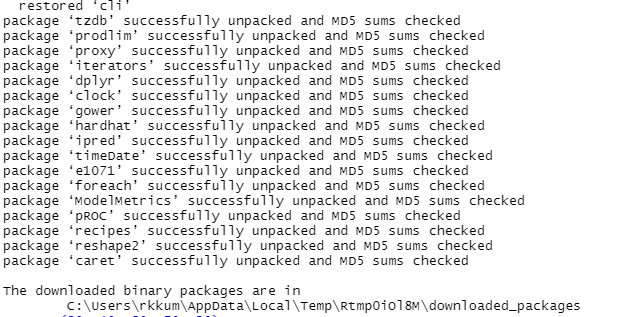
An output message is displayed like this it shows that other packages also installed that supports caret package

2. Prepare your data: Your data should be ready with the outcome variable and predicted values from a model or algorithm.

3. Calculate confusion matrix: Use the function “confusionMatrix()” from “caret” package to calculate the confusion matrix based on the actual and predicted values. The confusion matrix provides the necessary information for calculating sensitivity, specificity and predictive values.

Parameters in confusionMatrix() function:

Parameter	Description
data	This specifies the predicted values or labels
reference	This specifies the actual values or lables.
positive	This parameter specifies the positive class or category.
dnn	Allows you to provide names for the dimensions of the confusion matrix.
mode	It determines how the confusion matrix is calculated. It can take values such as “sens_spec”(default), “prec_rec”, etc.
“…”	this parameter allows you to pass additional arguments to the underlying “table()” function.

As of now, we don’t use all these parameters we need only data and reference parameters. The “confusionMatrix()” expects the factors used as input should be of the same levels. If the factors have different levels, it will result in an error. For example, If we are using binary classification there are only two levels they are 0 and 1. To ensure that both factors have the same levels, for that we can use the “factor()” function with the “levels” argument to specify the desired levels. Both actual and predicted variables store binary valued vectors with the same levels. “confusionMatrix()” is used to calculate the confusion matrix.

R

# prepare data
actual <- factor(c(0, 1, 0, 1, 0,
                   1, 0, 1, 0, 1),
                 levels = c(0, 1))
predicted <- factor(c(0, 0, 1, 1, 0,
                      0, 1, 1, 0, 0),
                    levels = c(0, 1))

# execute confusionMatrix()
confusion_matrix <- confusionMatrix(data = predicted,
                                    reference = actual)

Output:

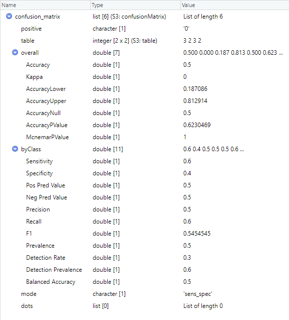
Calculate Sensitivity, Specificity and Predictive Values in CARET

The confusionMatrix() returns the list that contains 6 other lists of different lengths they are positive, table, overall, by class, mode, and dots each has its own type and respective values. This all provides a formatted summary of the confusion matrix and the performance metrics. The exact format of the output may vary depending on the version of the “caret” package and other packages loaded in your R environment.

Extract performance measures: the performance measures are already calculated in the “confusionMatrix()” function just have to extract them by using the “sensitivity()“, “specificity()“, “ppv()” functions from the caret package.

confusion_matrix holds the nested list that is returned by “confusionMatrix()” to extract values of sensitivity, specificity, positive predicted value, and negative predicted value we find all performance measures in the “byClass” list. So, we access them using confusion_matrix[[“byClass”]][[“Sensitivity”]] statement, similarly we will access Specificity, positively predicted value, and negative predicted value.

R

# prepare data
actual <- factor(c(0, 1, 0, 1, 0,
                   1, 0, 1, 0, 1),
                 levels = c(0, 1))
predicted <- factor(c(0, 0, 1, 1, 0,
                      0, 1, 1, 0, 0),
                    levels = c(0, 1))
# execute confusionMatrix()
confusion_matrix <- confusionMatrix(data = predicted,
                                    reference = actual)

# extract performance metrics
sens <- confusion_matrix[["byClass"]][["Sensitivity"]]
spec <- confusion_matrix[["byClass"]][["Specificity"]]
pos_prediction <- confusion_matrix[["byClass"]][["Pos Pred Value"]]
neg_prediction <- confusion_matrix[["byClass"]][["Neg Pred Value"]]

# print values
print(sens)
print(spec)
print(pos_prediction)
print(neg_prediction)

Output:

0.6
0.4
0.5
0.5

The sensitivity value is 0.6 which indicates 60% in the same way Specificity is 40%, the positive predicted value is 50% and the negative predicted value is 50% for the given actual and predicted class.

These metrics help in understanding the strengths and weaknesses of the model and can assist in making informed decisions based on the model’s performance in real-world applications.