Support Vector Machine Classifier Implementation in R with Caret package

One of the most crucial aspects of machine learning that most data scientists run against in their careers is the classification problem. The goal of a classification algorithm is to foretell whether a particular activity will take place or not. Depending on the data available, classification algorithms strive to provide answers to questions like whether a client is likely to leave or not, whether a YouTube viewer is likely to click on the suggested video or not, and if it will rain today or not. In this tutorial, we’ll use R programming language to create the Support Vector Machine Classifier, which will help us solve a classification issue.

Support Vector Machine (SVM)

To comprehend the idea behind the support vector machine, it is necessary to know that the algorithm groups the points on either side according to their homogeneous relationships using a line called a hyperplane. These points are said to be linearly separable if a straight line can divide them up. Look at the hyperplane in the following figure that linearly divides the symbols for something like the stars and sun.

Looking at the above image, one might be surprised to learn that we can draw a line in a different shape and location to create a border between these two shapes, as shown in the following image. This raises the question of how a support vector classifier machine should handle these conditions in order to model for the specific classification problems that are being presented.

The aforementioned issue for support vector classifiers can be resolved by using a maximum margin hyperplane – the lines that produce the greatest gap between the two classes. Look at the image below, which shows the relationships between the shapes and the maximum margin hyperplane.

The three blue-filled shapes are what are referred to as support vectors. They serve as a foundation for a potential MMH definition. What happens if the points cannot be separated linearly? How does the support vector machine handle issues of this nature? In the presence of the slack variable, which enables the machine to break some limitations and allow a limited number of points to enter restricted areas, nothing is impossible for the support vector classifier. In this case, the machine worked to reduce the overall cost of an algorithm.

Another related issue that a support vector machine could run into when modeling real-world categorization data is the extensive non linearity of one data. The kernel technique, a feature of the support vector classifier that enables us to manipulate those data easily to linearly separable data, is also a solution for this kind of problem from the machine. Look at the illustration below.

By stating this, let’s examine how this machine learning method will be used in practice. We will delve into R and its package caret, one of the most popular open source programming languages. Caret, which stands for classification and regression training, is a potent capability that enables you to use it to create an enormous number of models. Let’s get going.

Importing Packages

All required packages installations and importing can be done using below code,

R

# Code for installation of all necessary packages
install.packages("caret")
install.packages("ggplot2")
install.packages("GGally")
install.packages("psych")
install.packages("ggpubr")
install.packages("reshape")

# Code for importation of all necessary packages
library(caret)
library(ggplot2)
library(GGally)
library(psych)
library(ggpubr)
library(reshape)

Loading Data

Dataset includes the information about 768 women from a community close to Phoenix, Arizona, USA, may be found in the Pima Indian Diabetes Dataset, which was originally created by the National Institute of Diabetes and Digestive and Kidney Diseases. This tutorial is designed to categorize whether the patient outcome is diabetes or not depending on the data in the dataset. 

Let’s add the data to the code.

R

# Code
df <- read.csv("data/diabetes.csv")
head(df)

Output:

To check if there is any null values in our dataset.

R

# Code
sum(is.na(df))

Output:

0

To see the dimensions of our dataset.

R

# Code
dim(df)

Output:

768  9

Data Visualization 

To see the type of our data frame.

R

# Code
sapply(df, class)

Output:

R

# Code
summary(df) # to calculate the summary of our dataset

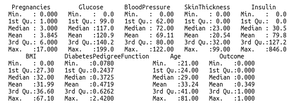
Summary of our Dataset

R

# Code
a <- ggplot(data = df, aes(x = Pregnancies)) +
    geom_histogram( color = "red", fill = "blue", alpha = 0.1) +
    geom_density()

b <- ggplot(data = df, aes(x = Glucose)) +
    geom_histogram( color = "red", fill = "blue", alpha = 0.1) +
    geom_density()

c <- ggplot(data = df, aes(x = BloodPressure)) +
    geom_histogram( color = "red", fill = "blue", alpha = 0.1) +
    geom_density()

d <- ggplot(data = df, aes(x = SkinThickness)) +
    geom_histogram( color = "red", fill = "blue", alpha = 0.1) +
    geom_density()

e <- ggplot(data = df, aes(x = Insulin)) +
    geom_histogram( color = "red", fill = "blue", alpha = 0.1) +
    geom_density()

f <- ggplot(data = df, aes(x = BMI)) +
    geom_histogram( color = "red", fill = "blue", alpha = 0.1) +
    geom_density()

g <- ggplot(data = df, aes(x = DiabetesPedigreeFunction)) +
    geom_histogram( color = "red", fill = "blue", alpha = 0.1) +
    geom_density()

h <- ggplot(data = df, aes(x = Age)) +
    geom_histogram( color = "red", fill = "blue", alpha = 0.1) +geom_density()
    ggarrange(a, b, c, d,e,f,g, h + rremove("x.text"),
          labels = c("a", "b", "c", "d","e", "f", "g", "h"),
          ncol = 3, nrow = 3)

Output:

R

# Code
ggplot(data = df, aes(x =Outcome, fill = Outcome)) +
    geom_bar()

Output:

Code to label our categorical variable as a factor

R

# Code to label our categorical variable as a factor
df$Outcome<- factor(df$Outcome,
                  levels = c(0, 1),
                  labels = c("Negative", "Positive"))

To select only numerical features from our dataset to plot boxplot.

R

out <- subset(df,
 select = c(Pregnancies,Glucose,
            BloodPressure,SkinThickness,
            Insulin,BMI,
            DiabetesPedigreeFunction,Age))

# Code for boxplot
ggplot(data = melt(out),
               aes(x=variable, y=value)) +
            geom_boxplot(aes(fill=variable))

Output:

To plot the correlation plot by using the psych package

R

corPlot(df[, 1:8])

Output:

Insights 

• In these findings, the mean of the variables necessary to predict the outcome variable—pregnancies, insulin, glucose, diabetes pedigree function, and age—is greater than the median. The mean is higher than the median because the data seem to be biased to the right.
• Our data’s histogram and boxplots support the conclusions of summary statistics.
• The correlation map, however, shows that the variables in our data do not strongly correlate with one another.

Based on the foregoing summary, how should we format the data? What would be the next step in this? I’ll let you work on this yourself.

Data preparation and Modelling

To split our dataset into training and validation

R

cutoff <- createDataPartition(df$Outcome, p=0.85, list=FALSE)
# select 15% of the data for validation
testdf <- df[-cutoff,]
# use the remaining 85% of data to training and testing the models
traindf <- df[cutoff,]

Let’s train the SVM model now.

R

# Code to train the SVM
set.seed(1234)
# set the 10 fold crossvalidation with AU
# to pick for us what we call the best model
control <- trainControl(method="cv",number=10, classProbs = TRUE)
metric <- "Accuracy"
model <- train(Outcome ~., data = traindf, method = "svmRadial",
                tuneLength = 8,preProc = c("center","scale"),
                   metric=metric, trControl=control)

To print the summary of the model.

R

# Code for model summary
model

Output:

Let’s plot the accuracy graph.

R

# Code
plot(model)

Output:

Let’s now evaluate the precision of our model. The confusion matrix will be used to forecast the accuracy.

R

# validate our model
predict <- predict(model, newdata = testdf)
confusionMatrix(predict, testdf$Outcome)

Output:

The accuracy on the validation set is 81.74%, according to the confusion matrix results, which suggests that our model can predict this dataset fairly well. With this, this tutorial comes to a close. I hope you learned something from and found it useful.