Implementing Agglomerative Clustering using Sklearn

Prerequisites: Agglomerative Clustering Agglomerative Clustering is one of the most common hierarchical clustering techniques. Dataset – Credit Card Dataset. Assumption: The clustering technique assumes that each data point is similar enough to the other data points that the data at the starting can be assumed to be clustered in 1 cluster. Step 1: Importing the required libraries

Python3

import pandas as pd
import numpy as np
import matplotlib.pyplot as plt
from sklearn.decomposition import PCA
from sklearn.cluster import AgglomerativeClustering
from sklearn.preprocessing import StandardScaler, normalize
from sklearn.metrics import silhouette_score
import scipy.cluster.hierarchy as shc

Step 2: Loading and Cleaning the data

Python3

# Changing the working location to the location of the file
cd C:\Users\Dev\Desktop\Kaggle\Credit_Card

X = pd.read_csv('CC_GENERAL.csv')

# Dropping the CUST_ID column from the data
X = X.drop('CUST_ID', axis = 1)

# Handling the missing values
X.fillna(method ='ffill', inplace = True)

Step 3: Preprocessing the data

Python3

# Scaling the data so that all the features become comparable
scaler = StandardScaler()
X_scaled = scaler.fit_transform(X)

# Normalizing the data so that the data approximately
# follows a Gaussian distribution
X_normalized = normalize(X_scaled)

# Converting the numpy array into a pandas DataFrame
X_normalized = pd.DataFrame(X_normalized)

Step 4: Reducing the dimensionality of the Data

Python3

pca = PCA(n_components = 2)
X_principal = pca.fit_transform(X_normalized)
X_principal = pd.DataFrame(X_principal)
X_principal.columns = ['P1', 'P2']

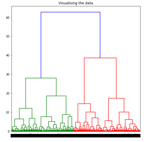
Dendrograms are used to divide a given cluster into many different clusters. Step 5: Visualizing the working of the Dendrograms

Python3

plt.figure(figsize =(8, 8))
plt.title('Visualising the data')
Dendrogram = shc.dendrogram((shc.linkage(X_principal, method ='ward')))

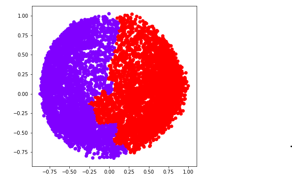
To determine the optimal number of clusters by visualizing the data, imagine all the horizontal lines as being completely horizontal and then after calculating the maximum distance between any two horizontal lines, draw a horizontal line in the maximum distance calculated. 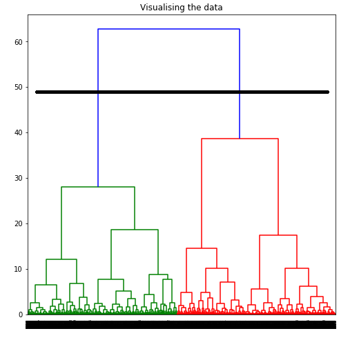The above image shows that the optimal number of clusters should be 2 for the given data. Step 6: Building and Visualizing the different clustering models for different values of k a) k = 2

Python3

ac2 = AgglomerativeClustering(n_clusters = 2)

# Visualizing the clustering
plt.figure(figsize =(6, 6))
plt.scatter(X_principal['P1'], X_principal['P2'],
           c = ac2.fit_predict(X_principal), cmap ='rainbow')
plt.show()

b) k = 3

Python3

ac3 = AgglomerativeClustering(n_clusters = 3)

plt.figure(figsize =(6, 6))
plt.scatter(X_principal['P1'], X_principal['P2'],
           c = ac3.fit_predict(X_principal), cmap ='rainbow')
plt.show()

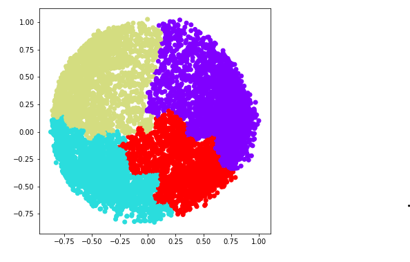
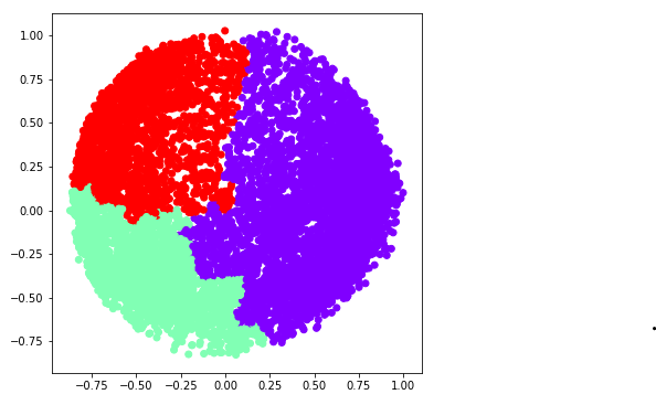c) k = 4

Python3

ac4 = AgglomerativeClustering(n_clusters = 4)

plt.figure(figsize =(6, 6))
plt.scatter(X_principal['P1'], X_principal['P2'],
            c = ac4.fit_predict(X_principal), cmap ='rainbow')
plt.show()

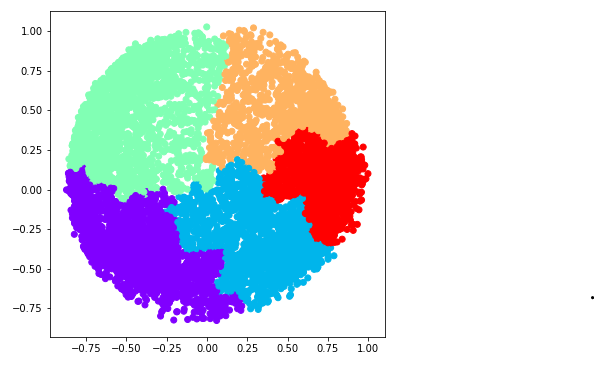
d) k = 5

Python3

ac5 = AgglomerativeClustering(n_clusters = 5)

plt.figure(figsize =(6, 6))
plt.scatter(X_principal['P1'], X_principal['P2'],
            c = ac5.fit_predict(X_principal), cmap ='rainbow')
plt.show()

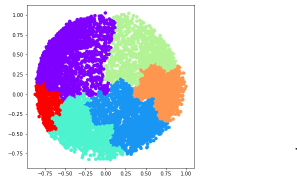
e) k = 6

Python3

ac6 = AgglomerativeClustering(n_clusters = 6)

plt.figure(figsize =(6, 6))
plt.scatter(X_principal['P1'], X_principal['P2'],
            c = ac6.fit_predict(X_principal), cmap ='rainbow')
plt.show()

We now determine the optimal number of clusters using a mathematical technique. Here, We will use the Silhouette Scores for the purpose. Step 7: Evaluating the different models and Visualizing the results.

Python3

k = [2, 3, 4, 5, 6]

# Appending the silhouette scores of the different models to the list
silhouette_scores = []
silhouette_scores.append(
        silhouette_score(X_principal, ac2.fit_predict(X_principal)))
silhouette_scores.append(
        silhouette_score(X_principal, ac3.fit_predict(X_principal)))
silhouette_scores.append(
        silhouette_score(X_principal, ac4.fit_predict(X_principal)))
silhouette_scores.append(
        silhouette_score(X_principal, ac5.fit_predict(X_principal)))
silhouette_scores.append(
        silhouette_score(X_principal, ac6.fit_predict(X_principal)))

# Plotting a bar graph to compare the results
plt.bar(k, silhouette_scores)
plt.xlabel('Number of clusters', fontsize = 20)
plt.ylabel('S(i)', fontsize = 20)
plt.show()

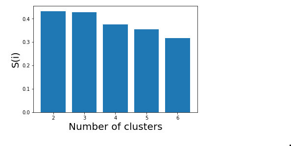Thus, with the help of the silhouette scores, it is concluded that the optimal number of clusters for the given data and clustering technique is 2.