What is State Space Analysis ?

The State Space analysis applies to the non-linear and time-variant system. It helps in the analysis and design of linear, non-linear, multi-input, and multi-output systems. Earlier the transfer function applied to the linear time-invariant system but with the help of State Space analysis, it is possible to find the transfer function of the non-linear and time-variant systems. In this article, we will study the State Space Model in control system engineering.

What is the State Space Analysis?

State Space Analysis is the graphical tool that is used to analyze and design the linear, non-linear, time-variant, time-invariant multi-input, multi-output system. It is used to describe the behavior of LTI systems. It describes the internal state of the system. There are various key components of the state space analysis which are as follows:

• State and State Variable
• State Vector
• State Space

State and State Variable

The state of a dynamical system is a set of minimal variables and the knowledge of these variables at t=t_o together with input for [Tex]t\geq t_{o} [/Tex] completely determines the behavior of the system for any time t. In other words, the compact representation of the previous history of the system is known as the State of the system.

The variables that contain the dynamic information of the system are known as State Variables.

State Vector

The ‘n’ set of state variables which describes the dynamic equations of the linear system, then it can be considered as N components of a vector q. The given below is the state vector of continuous system.

State Vector

State Space

When the coordinate axis of the N-dimensional space consist of q1-axis, q2-axis, …., qn-axis, it is known as state space. Any state can be represented by the point in the state space.

State Space Model

The single-input and single output continuous time LTI system is described by the differential equation which is given below:

[Tex]\frac{d^Ny(t)}{dt^N}+\frac{d^{N-1}y(t)}{dt^{N-1}}+….+a_{n}y(t)=x(t) [/Tex] —-(1)

The N state variables q₁(t), q₂(t), ….,q_n(t) is defined as:

q₁(t)=y(t) , …., q_n(t)= y^(n-1)(t)

where [Tex]y^k(t)=\frac{d^ky(t)}{dt^k} [/Tex] —–(2)

From equation (1) and equation (2)

[Tex]\dot{q_{n}(t)}= -a_{n}q_{1}(t)-a_{n-1}q_{2}(t)-…….-a_{1}q_{n}(t)+x(t) [/Tex] ——-(3)

and,

y(t)=q₁(t) —— (4)

The equation 3 and equation 4 can be expressed in the matrix form as given below where [Tex]\dot{q_{k}(t)}= \frac{dq_{k}(t)}{dt} [/Tex]:

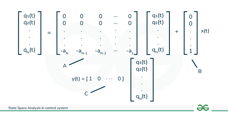
Matrix Form

Hence the final state equation will be:

[Tex]\dot{q(t)} = Aq(t)+Bx(t) [/Tex] —- (state equation)

[Tex]y(t)=Cq(t)+Dx(t) [/Tex] —- (output equation)

Transfer Function from State Space Model

The transfer function can be calculated using state space analysis. We will now see the procedure for calculating the transfer function.

The state equations of the LTI system are:

[Tex]\dot{x} = Ax+Bu [/Tex] —- (state equation (1))

[Tex]y=Cx+Du [/Tex] —- (output equation (2))

Applying Laplace Transform on both the sides of equation (1):

sx(s) = Ax(s)+Bu(s)

(sI-A)x(s) = Bu(s)

[Tex]x(s)= \frac{Bu(s)}{sI-A} [/Tex] —(3)

Applying Laplace Transform on both the sides of equation (2):

y(s) = Cx(s)+Du(s) —-(4)

Now, substituting the value of equation 3 into equation 4, we will get:

[Tex]y(s)= C\frac{Bu(s)}{sI-A} + du(s) [/Tex]

[Tex]\frac{y(s)}{u(s)} = \frac{C}{sI-A}B + D [/Tex] — (5)

where,

• A: system matrix (nxn)
• B: input matrix (nxm)
• C: output matrix (pxn)
• D: relevance of output with input matrix

The equation 5 represents the transfer function of the given system. With the help of this equation we can directly calculate the transfer function of the system.

State Transition Matrix and its Properties

State Transition Matrix

If the matrix is satisfying the linear homogenous state equation then the matrix is called state transition matrix. Linear homogenous state equation is described below:

[Tex]\dot{x(t)}=\frac{dx(t)}{dt} = Ax(t) [/Tex] —(1)

Let [Tex]\phi(t) [/Tex] be the state transition matrix then

[Tex]\frac{d\phi(t)}{dt} =A\phi(t) [/Tex] —(2)

If [Tex]\phi(t) [/Tex] is the state transition matrix, it will satisfy the given condition:

[Tex]x(t)=\phi(t)x(0) [/Tex] —– (3)

Taking the laplace transform of the equation (1):

sx(s)-x(0) = Ax(s)

x(s)(sI-A) = x(0)

x(s) = (sI-A)^-1x(0)

Taking the inverse laplace transform of the above equation:

x(t) = L^-1[(sI-A)^-1x(0)]

The state transition matrix is:

Φ(t) = L^-1[(sI-A)^-1] = e^At

State Transition Matrix Properties

There are five important properties of state transition matrix:

1. ϕ(t) = I (I is the identity matrix)
2. ϕ(t) = e^At = (e^-At)^-1 = [ϕ(-t)]^-1
3. ϕ(t₂-t₀) = ϕ(t₂-t₁)ϕ(t₁-t₀)
4. ϕ(t-t₀) = ϕ(t) ϕ^-1(t₀)
5. ϕ(t+t₀) = ϕ(t) ϕ(t₀)

Controllability and Observability

Controllability

The system is controllable when the desired output is obtained by applying the specific controlled input. It is the ability to control the state of the system. The controllability of the system can be checked using the Kalam Test. The given below is the condition for the controllability:

Q₀ = [B AB A²B ….. A^n-1B]

If the determinant of Q₀ is not equal to 0 then the system is controllable.

[Tex]|Q_{0}| \neq0 [/Tex] —- (system is controllable)

|Q₀| = 0 —– (system is un-controllable)

Observability

It is the system’s ability to measure or observe the system state. If the internal state of the system is determined using the input and output signals during a finite interval of time then the system is said to be observable. The observability of the system can be checked using the Kalam Test. The given below is the condition for the observability:

Q₀ = [C^T A^TC^T ….. (A^T)^n-1C^T]

Note: A^T,C^T means transpose of the respective matrix

If the determinant of Q₀ is not equal to 0 then the system is controllable.

[Tex]|Q_{0}| \neq0 [/Tex] —- (system is observable)

|Q₀| = 0 —– (system is not observable)

Solved Example on State Space Analysis

Example: Obtain the state space equation of the following differential equation:

[Tex]\frac{2d^3y}{dt^3}+\frac{4d^2y}{dt^2}+\frac{6dy}{dt}+8y=10u(t) [/Tex]

Solution

Triple derivative –> 3 variables

[Tex]x_{1}=y [/Tex]

[Tex]x_{2}=\frac{dy}{dt}=\dot{x_{1}} [/Tex]

[Tex]x_{3}=\frac{d^2y}{dt^2}=\dot{x_{2}} [/Tex]

[Tex]\dot{x_{3}}=\frac{d^3y}{dt^3} [/Tex]

[Tex]\frac{d^3y}{dt^3} = 5u(t)-\dot{\dot{{2y}}}-3\dot{y}-4y [/Tex]

[Tex]\frac{d^3y}{dt^3} = 5u(t)-2x_{3}-3x_{2}-4x_{1} [/Tex]

The final solution is given below:

Final Solution

Advantages and Disadvantages of State Space Analysis

There are some list of Advantages and Disadvantages of State Space Analysis given below :

Advantages

1. It provides an easy way to find the transfer function of the system where Laplace Transform and z-transform cannot be applied.
2. It applies to the non-linear and time-variant systems as well.
3. It helps in analyzing the behavior of the system.
4. It helps in the designing of the controllers. It is helpful in pole placement techniques.
5. It can handle multi-input and multi-output systems easily.

Disadvantages

1. State Space analysis become complex for large-scale systems because it involves a high number of state variables and equations.
2. It is less preferred in discrete-time systems.
3. It requires a better understanding of the advanced mathematical tools and numerical techniques because State Space analysis uses this technique for computation.

Applications of State Space Analysis

1. It finds its application in the modeling of mechanical systems like manufacturing processes, robotic arms, and many more.
2. It helps design the flight control system. With the help of state space analysis dynamic behaviour of the aircraft can be studied properly.
3. It is used in robotics technology to study the arm’s motion and stability using the transfer function
4. To improve the reliability of the control power system, the state space analysis is used.

Conclusion

The article deals with the State Space Analysis model which is used in the control system. It is useful to find the transfer function of the non-linear, time-variant, multi-input, and multi-output systems. It provides an easy way for the system analysis. In this article, we have studied the concept of state space analysis, the calculation of the transfer functions, its application, advantages, and disadvantages.

FAQs on State Space Analysis in Control System

1. How does the controllability impact the designing of the system?

Controllability can impact the system design because it ensures the how controller can manipulate the behavior of the system according to our desired output.

2. How does pole-zero analysis related to state-space representation?

Pole-zero analysis is applied on the transfer function of the system to find the stability of the system. While State Space analysis is used to find the transfer function of the system.

3. Can a system have multiple state-space representations?

Yes, a system can have multiple state-space representations.