Control Systems – Root Locus

The root locus is a procedure utilized in charge framework examination and plan. It centers around figuring out how the roots (or posts) of the trademark condition of a control framework change as a particular boundary, frequently the control gain, is changed. This graphical technique is especially useful in deciding the soundness and transient reaction of the framework.

Root Locus

The root locus is a graphical strategy utilized in charge frameworks designing to break down the way of behaving of a framework’s shut circle posts as a boundary, ordinarily an addition, is fluctuated. It assists specialists and control framework originators with understanding what changes in framework boundaries mean for strength and execution.

Key Points About the Root Locus

• System Transfer Function: Find the trademark condition of the framework, not set in stone by setting the denominator of the exchange capability equivalent to nothing. The trademark condition assists us with tracking down the shafts of the framework.
• Open-Loop Transfer Function: The system’s transfer function is separated into its open-loop and closed-loop components. The open-loop transfer function describes the system without any feedback control.
• Characteristics Equation: Find the trademark condition of the framework, not entirely set in stone by setting the denominator of the exchange capability equivalent to nothing. The trademark condition assists us with tracking down the shafts of the framework.
• Root Calculation: Ascertain the roots (shafts) of the trademark condition for each worth of the boundary. These roots are perplexing numbers, and their area in the mind-boggling plane shows the security and conduct of the shut circle framework.
• Parameter Variation: Differ a boundary, frequently the increase (K), while keeping any remaining boundaries consistent. This boundary addresses the regulator gain as a rule.
• Design: Utilize the root locus plot to plan a regulator that accomplishes the ideal shut circle framework conduct. Change the boundary esteem (frequently the addition) to put the shut circle shafts in the ideal areas.
• Plotting: Plot these roots in the complicated plane for various upsides of the boundary. As you change the boundary, the roots will move, and the root locus plot will show the directions of these roots.
• Analysis: Investigate the root locus plot to decide how the shut circle framework’s security and execution change with differing boundary values. Central issues to note incorporate the area of posts concerning the dependability district, damping proportion, and normal recurrence.

Angle Condition and Magnitude Condition of Root Locus

On moving further , the two terms are explained –

Angle Condition: The point condition relates the places where open-circle posts and zeros withdraw and show up at focuses on the root locus. The key idea is that the amount of the points of takeoff from open-circle shafts to the locus should rise to the amount of the points of landing in open-circle zeros from the locus, and this aggregate should be an odd different of 180 degrees (π radians).

Angle Condition Formula:

Σ(θ_departure) – Σ(θ_arrival) = (2n + 1) * π radians

Where:

• θ_departure: The angle from an open-loop pole to a point on the root locus.
• θ_arrival: The angle from an open-loop zero to a point on the root locus.
• n: An integer representing the number of iterations around the root locus. The summation should be performed as the locus moves from one open-loop pole to the next.

Magnitude Condition: The extent condition relates the sizes of the open-circle move capability at guides on the root locus toward the increase (K) and the separation from these focuses to the closest open-circle posts or zeros. The size condition decides the extent of the framework’s reaction at different focuses on the locus.

Magnitude Condition Formula:

|G(s)| = |K * G_o(s)|

Where:

• |G(s)|: The magnitude of the open-loop transfer function at a point on the root locus.
• K: The control gain (parameter under consideration).
• G_o(s): The open-loop transfer function.
• Additionally, the phase angle (φ) at any point on the root locus can be expressed as: φ = Σ(θ_departure) – Σ(θ_arrival)

The magnitude condition provides information about how the magnitude of the system’s response at various points on the root locus changes with varying gain (K).

Stability Analysis

Engineers utilize the root locus to survey framework dependability. Assuming every one of the posts of the shut circle framework lie in the left-half of the perplexing plane (i.e., they have negative genuine parts), the framework is steady. On the other hand, assuming that any post crosses into the right-half of the perplexing plane, the framework becomes shaky.

Performance Analysis

The root locus also provides insights into system performance. For instance:

• Damping proportion (ζ) can be derived from the point of flight or appearance of the root locus branches as they approach asymptotes.
• Regular recurrence (ωn) can be assessed in light of the distance between posts along a branch.
• Overshoot and settling time attributes can be anticipated in light of post areas.

Rules and Guidelines

• Shafts move towards parts of the root locus as the addition boundary (K) increments.
• The parts of the root locus start at open-circle shafts (posts of the framework without input) and end at open-circle zeros (zeros of the framework without criticism).
• The root locus plot is balanced regarding the real axis.
• The number of branches in the root locus is equal to the number of open-loop poles.
• Branches cross the genuine pivot where the increase boundary (K) causes the denominator of the shut circle move capability to rise to nothing.

Advantages

• Model-Free Analysis: Root locus investigation is a model-based approach yet doesn’t need an exact model of the framework. This is especially worthwhile while managing complex or ineffectively figured out frameworks, as it takes into consideration framework investigation and plan without exact numerical models.
• Geometric Insight: Root locus gives mathematical understanding into the connections between control boundaries and framework conduct. Specialists can naturally comprehend what changes in gain mean for post areas, which can direct the plan cycle.
• Complex Systems: Root locus is material to frameworks with complex exchange capabilities, incorporating those with different shafts, zeros, and higher-request elements. It can work on the examination and plan of such frameworks.
• Educational Value: Root locus is a fantastic instructive device that assists understudies and designers with fostering a more profound comprehension of control framework hypothesis and how control boundaries impact framework reaction.
• Control Tuning: The strategy is broadly utilized in functional control framework tuning, permitting specialists to enhance regulator boundaries for certifiable applications, further developing framework execution, and decreasing motions or overshoot.
• Adaptive Control: Root locus examination can be applied in versatile control frameworks, where the control boundaries need to adjust to evolving conditions. It gives experiences into how the control boundaries ought to develop to keep up with framework security and execution.

Limitations

While root locus is a useful asset, it has impediments. It expects direct time-invariant frameworks, and it may not completely catch the impacts of nonlinearities or time delays. Moreover, it fundamentally manages single-input, single-yield (SISO) frameworks.

ROOT LOCUS

The root locus strategy is a central procedure in control frameworks designing. It gives a graphical portrayal of how a framework’s posts change with varieties in a control boundary, empowering specialists to plan regulators that meet strength and execution details. It’s an important instrument for understanding and enhancing the way of behaving of dynamic frameworks.

Step by Step Procedure of Creating Root Locus Plot

The following steps are used for creating the root locus plot :

• Start with the Open-Loop Transfer Function

Start with the open-circle move capability (otherwise called the framework move capability), which addresses the connection between the information and result of the control framework. This move capability commonly takes the form:

G(s)= D(s)/N(s)

Where:

G(s) is the transfer function of the system.
N(s) is the numerator polynomial.
D(s) is the denominator polynomial.

• Determine the Characteristic Equation

The trademark condition is inferred by setting the denominator $D(s)$ equivalent to nothing. It addresses the shut circle framework’s way of behaving and solidness. The trademark condition is normally of the form:

1+KG(s)=0

Where:

K is the control​ parameter (often the gain of a controller).
G(s) is the open-loop transfer function.

• Identify the Open-Loop Poles and Zeros

Track down the posts (foundations) of the denominator polynomial D(s) and any open-circle zeros by settling the condition D(s) = 0 and N(s) = 0, separately. These shafts and zeros are the beginning stages for building the root locus.

• Determine the Number of Branches:

The root locus will consist of as many branches as there are open-loop poles. Each branch starts at an open-loop pole.

• Calculate the Breakaway and Break-in Points

There the root locus branches move towards or away from one another. To work out the breakaway and break-in focuses, separate the trademark condition as for s and settle for s to find the places where the subordinate equivalents zero. These focuses show where branches start or end.

• Determine Asymptotes

Find the asymptotes that depict the overall heading where the root locus branches move as the addition boundary K fluctuates. Asymptotes can be determined utilizing the accompanying equations:

Number of Asymptotes = Number of Poles – Number of Zeros

Angle of Asymptotes (theta_a) = frac{(2n + 1)\pi}{N-P}$, where n is an integer from 0 to (N – P – 1), N is the number of poles, and P is the number of zeros.

Centroid of Asymptotes (point where they intersect) = frac{\sum \text{Poles} – \sum \text{Zeros}}{N-P}.

• Draw the Root Locus

Beginning at the open-circle shafts, draw the root locus branches as the increase boundary $K$ shifts from zero to vastness. Follow the asymptotes’ bearings and move toward any zeros.

• Check for Crossing the Imaginary Axis

The root locus crosses the fanciful pivot if and provided that there is an odd number of posts and zeros to one side of an odd number of asymptotes. This crossing decides the framework’s security.

• Calculate the Gain for Desired Pole Locations

When you have the root locus plot, you can choose an ideal shut circle shaft area for the framework (e.g., wanted damping proportion and regular recurrence). Then, find the comparing worth of the increase boundary $K$ that puts the posts at the ideal areas utilizing the root locus plot.

• Evaluate Performance

Analyze the stability and performance characteristics of the closed-loop system for the selected gain value. This includes assessing overshoot, settling time, and transient response.

Example of Root Locus

The following is the example of root locus-

Draw the root locus diagram for a closed loop system whose loop transfer function is given by

G(s)H(s) = K/s(s + 3)(s + 6)

Solution:

Step 1: Finding the poles, zeroes, and branches.

The denominator of the given transfer function signifies the poles and the numerator signifies the zeroes. Hence, there are 3 poles and no zeroes.

Poles = 0, -3, and -6

Zeroes = No zero

P – Z = 3 – 0 = 3

There are three branches (P – Z) approaching to infinity and there are no open loop zeroes. Hence infinity will be the terminating point of the root locus.

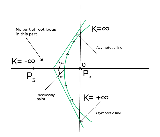
Step 2: Angle of asymptotes.

Angle of such asymptotes is given by:

= (2q + 1)180 / P – Z

q = 0, 1, and 2

For q = 0,

Angle = 180/3 = 60 degrees

For q = 1,

Angle = 3×180/3 = 180 degrees

For q = 2,

Angle = 5×180/3 = 300 degrees

Step 3: Centroid

The centroid is given by:

σ = Σ Real part of poles of G(S)H(S) – Σ Real part of Zeros of G(S)H(S)/P-Z

= 0 – 3 – 6 – 0/3

= -9/3

= -3

Thus, the centroid of the root locus is at -3 on the real axis.

Step 4: Breakaway point

We know that the breakaway point will lie between 0 and -3. Let’s find the valid breakaway point.

1 + G(s)H(s) = 0

Putting the value of the given transfer function in the above equation, we get:

1 + K/s(s + 3)(s + 6) = 0

s(s + 3)(s + 6) + K = 0

s(s^2 + 15^s + 50) + K = 0

s^3 + 9s^2 + 18^s + K = 0

K = – s^3 – 9s^2 – 18^s

Differentiating both sides,

Dk/ds = – (3s^2 + 18^s + 18) = 0

3s^2 + 18^s + 18 = 0

Dividing the equation by 3, we get:

s^2 + 6^s + 6 = 0

Now, we will find the roots of the given equation by using the formula:

-b+-√(b^2-4ac)/2ac

Using the value, a = 1, b = 6, and c = 6

The roots of the equation will be -1.268 and -4.732.

Among the two roots, only -1.268 lie between 0 and -3. Hence, it will be the breakaway point.

Let’s verify by putting the value of the root in the equation K = – s^3 – 9s^2 – 18^s.

K = – (-1.268)^3 – 9(-1.268)^2 – 18(-1.268)

K = 9.374.

The value of K is found to be positive. Thus, it is a valid breakaway point.

Step 5: Intersection with the negative real axis.

Here, we will found the intersection points of the root locus on the imaginary axis using the Routh Hurwitz criteria using the equation s^3 + 9s^2 + 18^s + K = 0

The Roth table is shown below:

s^3	1	18
s^2	9	k
s	9*18 – 1k/k = 162 – k/k	0
s^0	k

From the third row s, 750 – K/K = 0

162 – K = 0

K = 162

From the second row s2,

9 s^2 + K = 0

Putting the value of Kin the above equation, we get:

9 s^2 = -162

s2 = -162/9

s2 = -18

s = j4.242 and -j4.242

Both the point lies on the positive and negative imaginary axis.

Step 6: There are no complex poles present in the given transfer function. Hence, the angle of departure is not required.

Step 7: Combining all the above steps.

The root locus thus formed after combining all the above steps is shown below:

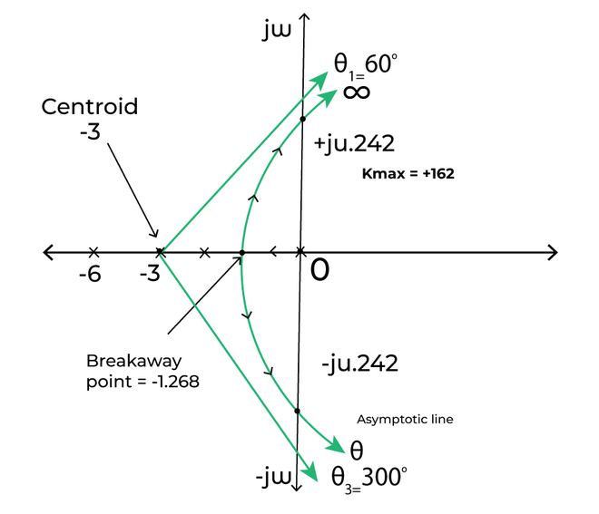
construction of root locus

Step 9: Stability of the system

The system can be stable, marginally stable, or unstable. Here, we will determine the system’s stability for different values of K based on the Routh Hurwitz criteria discussed above.

The system is stable if the value of K lies between 0 and 162. The root locus at such a value of K is in the left half of the s-plane. For a value greater than 162, the system becomes unstable, and it is because the roots start moving towards the right half of the s-plane. But, at K = 162, the system is marginally stable.

We can conclude that stability is based on the location of roots in the left half or right half of the s-plane.

Conclusion

In conclusion, the root locus procedure is a strong and flexible technique in the field of control framework designing. Its benefits incorporate its capacity to give an unmistakable visual portrayal of how a control framework’s conduct changes with fluctuating boundaries, its part in deciding framework dependability and execution, and its instructive incentive for grasping control hypothesis standards. Root locus examination is material to many frameworks, incorporating those with complex elements, and it is helpful for both hypothetical investigation and useful control framework plan and tuning. By offering bits of knowledge into the connections between control boundaries and framework conduct, the root locus strategy keeps on being a significant device for designers and understudies in the field of control systems.

FAQs on Root locus

1. What is the significance of the root locus method in control systems design?

The root locus strategy is fundamental in control frameworks plan since it gives a graphical portrayal of how the posts of a framework change as a control boundary, ordinarily the addition, is differed. Creators can utilize it to comprehend and streamline a framework’s dependability and execution. It helps answer questions like where to put shafts for wanted execution and what framework boundaries mean for steadiness.

2. How do I determine the stability of a system using the root locus plot?

A framework is steady in the event that all the shut circle posts (found from the root locus plot) have negative genuine parts. In the root locus, in the event that all parts of the plot lie in the left 50% of the mind boggling plane, the framework is steady. In the event that any branch crosses into the right a portion of, the situation becomes unsteady.

3. Can I use the root locus method for systems with multiple inputs and outputs (MIMO systems)?

The root locus strategy is basically intended for single-input, single-yield (SISO) frameworks, where there’s one info and one result. For MIMO frameworks, the augmentation of the root locus technique turns out to be more perplexing and more uncommon. Designs frequently utilize different strategies, for example, eigenvalue investigation and state-space techniques, for MIMO frameworks.

4. What if the open-loop transfer function has time delays? Can I still use the root locus method?

The root locus strategy is generally appropriate to straight time-invariant (LTI) frameworks. Assuming your open-circle move capability incorporates time delays, it can in any case be broke down utilizing root locus, yet the graphical translation becomes testing. You might have to utilize PC programming or mathematical strategies to deal with time delays really.