Construction of Root Locus

The Root Locus is the Technique to identify the roots of Characteristics Equations Within a Transfer Function. It Follows the Process of Plotting the roots on a graph, Showcasing their Variations across Different Parametric Values. In this article, we will be going through What is Root Locus?, Angle and Magnitude Conditions, Construction Rules of Root Locus, and At last we will solve the Examples.

What is Root Locus?

Root Locus is a method to find the roots of characteristic equations of the transfer function and to plot these roots in the graph for all the different parametric values. The roots are found for changing the different values of parameters and then plotted in the graph. Mostly these parametric values are the gain of the open loop transfer function but we can use any other variable also. We find the roots by varying the gain from 0 to infinite of the open loop transfer function.

The root locus is the graphical method of plotting the locus of roots in the s – s-plane for characteristic equation by the varying gain (k) from 0 to infinite. Through root locus, we can find the stability of the system.

Angle and Magnitude Condition

Angle and Magnitude conditions are important conditions for the construction of root locus.

The closed-loop transfer function for the given block diagram is

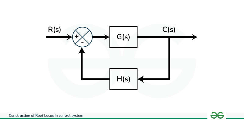
Closed Loop

C(s) / R(s) = G(s) / 1 + G(s) H(s)

Characteristic equation for above transfer function is

1 + G(s) H(s) =0

G(s) H(s) = -1

Here G(s) H(s) is complex part and it can be written in terms of magnitude and angle part

Angle Condition

Phase angle of G(s) H(s) is

∠G(s)H(s) = tan^-1 ( 0 / -1 ) = (2 n + 1 ) π , where n = 0, 1, 2, ……… (1)

Phase of open loop transfer function is odd multiple of 180⁰ at angle condition point.

Magnitude Condition

|G(s)H(s)|= 1 ……… (2)

Magnitude of open loop transfer function becomes 1 at Magnitude condition Point.

Equation 1 and 2 is also known as EVAN ‘ S CONDITION .

The value of s is roots of characteristic equation is if it satisfy both Angle and Magnitude condition.

Construction Rules of Root Locus

Following are the rules which need to be follow step by step for construction of Root Locus .

RULE 1 : Write down the characteristic equation 1 + G(s) H(s) = 0 and find open loop poles and zeros . Plot these open loop poles and zeros in s – plane . Root Locus start from open loop poles ( k=0 ) and ends at open loop zeros or infinite ( k= infinite) .

RULE 2 : Determine the number of branches of Root Locus , N

N = P if P > Z (if number of poles is grater than number of zeros than total number of branches is equal to number of poles.)

N = Z if P < Z (if number of zeros is grater than number of poles than total number of branches is equal to total number of zeros.)

N = P = Z if P = Z

where N = number of branches ; P = number of Poles ; Z = number of Zeros .

RULE 3 : The existence of root locus on a section of real axis is confirmed if sum of open loop poles and zeros to right of that point is odd number.

RULE 4 : Find Break away or Break in Point of root locus . It can be find out by writing the k in term of characteristic equation in s and then differentiating with respect to s and putting equals to 0 and solve for s .

1 + G(s) H(s) = 0

dk / ds =0

When two poles are placed adjacent to each other and and there exist root locus in between them then there must be minimum one Break Away Point between them.

When two zeros are placed adjacent to each other and and there exist root locus in between them then there must be minimum one Break In Point between them.

RULE 5 : Find Centroid point . Centroid is point where asymptotes intersect real axis . It is given as .

x = ( ∑ Real Part of pole − ∑ Real Part of Zeroes ) / (P -Z )

RULE 6 : Find the angle of Asymptotes . It can be determined from below given formula .

θ = ( 2 m + 1 ) 180⁰ / ( P -Z ) ; where m = 0 , 1 , 2 , 3 , …. , P- Z – 1

RULE 7 : To determine value of k and point at which root locus intersect imaginary axis we apply Routh Array Criteria in characteristic equation and find the value of k by solving auxiliary equation .

RULE 8 : Angle of departure is to be find out only for complex poles and its conjugate .

ϕ_d = 180⁰ – ( ϕ_p – ϕ_z ) ; where ϕ_d = Angle of departure , ϕ_P = sum of all the angle substituted to that pole by remaining poles , ϕ_Z = sum of all the angle substituted to that pole by remaining zeros.

RULE 9 : Angle of Arrival is to be find out only for complex zeros and its conjugate.

ϕ_a = 180⁰ + ( ϕ_P – ϕ_Z ) ; where ϕ_a = Angle of departure , ϕ_P = sum of all the angle substituted to that zero by remaining poles , ϕ_Z = sum of all the angle substituted to that pole by remaining zeros.

Effects of adding Open Loop Poles and Zeros on Root Locus

By adding open loop Poles and Zeros the Root Locus can be shifted in s plane . Following are the effects of adding open loop poles and zeros .

1. By adding open loop poles in transfer function , the root locus shift towards right side of s plane . Therefore the stability of system decreases .
2. By adding open loop zeros in transfer function , the root locus shift towards left side of s plane . Therefore the system stability increases.

Therefore we can add zeros and poles in transfer function as per requirement .

To Find Stability of system from Root Locus

Following are the criteria to find stability of system from Root Locus

1. If any branch of Root Locus is always in left hand side of s plane than system is stable.
2. If any branch of Root Locus is always in right hand side of s plane than the system is always unstable.
3. If any branch of Root Locus crosses imaginary axis than it is conditionally stable.
4. If any branch of Root Locus is always on imaginary axis than system is marginally stable.

Stability Plane

Solved Example of Root Locus

Draw the root locus for the open loop transfer function of unity feedback control system given below

G (s) H(s) = K / s (s+1) (s+3)

SOLUTION

STEP 1 : Open loop Poles and Zeros

s (s+1) (s+3) = 0

s= 0 ,-1 , -3 (poles)

There is no zeros

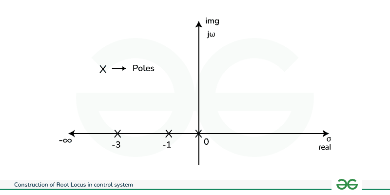
Diagram 1

STEP 2 : Number of branches of Root Locus , N

N = P = 3

STEP 3 : Existence of root locus on real axis , as per the rule the existence of root locus on real axis is (-∞ to -3 ) , (-1 to 0)

Diagram 2

STEP 4 : Break away Point

CE can be expressed as 1+ G(s) H(s) = 0

1 + k / s (s+1)(s+3) = 0

k = -s³ – 4s² – 3s

dk / ds = – (3s² + 8s + 3)

dk / ds = 0

=> -( 3s² + 8s + 3 ) =0

s = -0.45 , -2.21 (neglect)

STEP 5 : Centroid point , x = [ 0+ (-1) + (-3) ] – 0 / (3 – 0)

x = – 1. 33

STEP 6 : Angle of Asymptotes

θ = ( 2 m + 1 ) 180⁰ / ( P -Z ) ; where m = 0 , 1 , 2 {here P-Z-1 =2}

θ = 60⁰ , 180⁰ , 300⁰

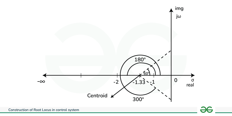
Diagram 3

STEP 7 : Intersection with imaginary axis by applying Routh Array Criteria

s3	1	3
s2	4	k
s1	(12 – k )/ 4	0
s0 = 1	k	0

12 – k / 4 =0

=> k = 12

auxiliary equation is 4s² + k =0

=> 4s² + 12 =0

=> s = 1.73 j , – 1.73 j

Since there is no complex poles and zeros of transfer function therefore there is no angle of departure and arrival .

Root Locus of given transfer function is as below

Diagram 4

Applications of Root Locus

Following are the some of the applications of Root Locus

• Used to do the analyses of Frequency response of system .
• Used in Lead and Lag compensation design .
• Used to find stability of system .
• Used in servo motor system for designing of controller .

Advantages of Root Locus

Following are the some of the advantage of Root Locus

• We can find the stability of system from Root Locus .
• Gain Margin , Phase margin can be determined from Root Locus .
• Performance of the system can be predicted through Root Locus .
• We can find Roots of Characteristic equation using angle and Magnitude condition.
• It is easy to implement .

Disadvantages of Root Locus

Following are the some of the disadvantage of Root Locus

• Root Locus technique can be applied only to Linear Time Invariant system .
• It is not suitable for Discrete Time System .
• Used only for the analyses of Closed Loop feedback system .
• It become more complex for multiple input output system .
• Time delay system is hard to analyze through it .

Conclusion

Root Locus Technique is very important method for the designing and the analysis of control system .Through this we get to know about the stability of system by plotting open loop zeros and poles of transfer function and by varying k parameter or gain parameter of system . It is also helpful for doing the performance analysis of the system . By plotting open loop poles and zeros we also get to know about their contribution in stability of system . We can also modify and add open loop poles and zeros to make system stable , unstable , conditional stable or marginal stable as per our needs.

FAQs on Root Locus

1. Root Locus is symmetric about which axis?

Root Locus is always symmetric about Real axis .

2. What do you mean by Asymptotes ?

Asymptotes are Root Locus branches or the path along which Root Locus moves towards infinity .

3. What is Break Away Point ?

The point at which Root Locus branch leaves the real axis is called Break Away Point .

4. What is Break In Point ?

The point at which Root Locus branch enters into to real axis it is called Break In Point .