SARIMA (Seasonal Autoregressive Integrated Moving Average)

Last Updated : 17 Nov, 2023

Time series data is all around us, from stock prices and weather patterns to demand forecasting and seasonal trends in sales. To make sense of this data and predict future values, we turn to powerful models like the Seasonal Autoregressive Integrated Moving Average, or SARIMA. In this article, we will unravel the mysteries of SARIMA models, to forecast the monthly sales.

Understanding SARIMA

SARIMA, which stands for Seasonal Autoregressive Integrated Moving Average, is a versatile and widely used time series forecasting model. It’s an extension of the non-seasonal ARIMA model, designed to handle data with seasonal patterns. SARIMA captures both short-term and long-term dependencies within the data, making it a robust tool for forecasting. It combines the concepts of autoregressive (AR), integrated (I), and moving average (MA) models with seasonal components.

The Components of SARIMA

To grasp SARIMA, let’s break down its components:

Seasonal Component: The “S” in SARIMA represents seasonality, which refers to repeating patterns in the data. This could be daily, monthly, yearly, or any other regular interval. Identifying and modelling the seasonal component is a key strength of SARIMA.
Autoregressive (AR) Component: The “AR” in SARIMA signifies the autoregressive component, which models the relationship between the current data point and its past values. It captures the data’s autocorrelation, meaning how correlated the data is with itself over time.
Integrated (I) Component: The “I” in SARIMA indicates differencing, which transforms non-stationary data into stationary data. Stationarity is crucial for time series modelling. The integrated component measures how many differences are required to achieve stationarity.
Moving Average (MA) Component: The “MA” in SARIMA represents the moving average component, which models the dependency between the current data point and past prediction errors. It helps capture short-term noise in the data.

Seasonal Differencing

Before we jump into SARIMA, it’s essential to understand seasonal differencing. Seasonal differencing is the process of subtracting the time series data by a lag that equals the seasonality. This helps remove the seasonal component and makes the data stationary, allowing for more straightforward modeling. Seasonal differencing is often denoted as “D” in SARIMA.

The SARIMA Notation

SARIMA(p, d, q)(P, D, Q, s):
AR(p): Autoregressive component of order p
MA(q): Moving average component of order q
I(d): Integrated component of order d
Seasonal AR(P): Seasonal autoregressive component of order P
MA(Q): Seasonal moving average component of order Q
Seasonal I(D): Seasonal integrated component of order D
s: Seasonal period

The mathematical representation of SARIMA is as follows:

$(1 - \phi_1B )(1 - \Phi_1B^{s})(1 - B)(1 - B^s)y_t = (1 + \theta_1B )(1 + \Theta_1B^s)\varepsilon_t$

Where,

$y_t$ is the observed time series at time $t$,
B is the backward shift operator, representing the lag operator (i.e., $By_t = y_{t-1}$ )
$\phi_1$ is the non-seasonal autoregressive coefficient,
$\Phi_1$ is the seasonal autoregressive coefficient,
$\theta_1$ is the non-seasonal moving average coefficient,
$\Theta_1$ is the seasonal moving average coefficient,
s is the seasonal period,
$\varepsilon_t$ is the white noise error term at time t.

Lеt’s go through each component of the equation:

Autoregressive (AR) Component: The autoregressive non-seasonal component represented by $(1 - \phi_1B )$ captures the relationship between the current observation and a certain number of lagged observations (previous values in the time series). The B term represents the backshift operator is commonly used in time series analysis. It represents the lag operator, which shifts the time series backward by a certain number of time period. The order of the autoregressive component, denoted by (p), determines the number of past values considered in the model.
Seasonal Autoregressive (SAR) Component: Thе seasonal autoregressive component is represented by $(1 - \Phi_1B^{s})$ This component captures the relationship between the current observation and a certain number of lagged observations at seasonal intervals. Thе $B^s$ term represents the backshift operator applied to the seasonal lagged observations.
Non-Seasonal Differencing Component: The non-seasonal differencing component is represented by $(1 - B)$ , where d is the order of non-seasonal differencing. This component is used to make the time series stationary by differencing it a certain number of times.
Seasonal Differencing Component: Thе seasonal differencing component is represented by $(1 - B^s)$ , where D is the order of seasonal differencing and. This component is used to make the time series stationary by differencing it at seasonal intervals.
Observed Time Series: Thе observed time series is denoted by yₜ. It represents the historical data that we have and want to forecast.
Moving Average (MA) Component: The moving average component is represented by $(1 + \theta_1B )$ . This component captures the relationship between the current observation and the residual errors from a moving average model appliеd to lagged observations.
Seasonal Moving Average (SMA) Component: The seasonal moving average component is represented by $(1 + \Theta_1B^s)$ . This component captures the relationship between the current observation and the residual errors from a moving average model applied to lagged observations at seasonal intervals.
Error Term: The error term is denoted by $\varepsilon_t$ . It represents the random noise or unexplained variation in the time series.

Thе SARIMA model is estimated by fitting the model to the historical data and then using it to forecast future values.

Use Cases for SARIMA

SARIMA models find applications in various domains, including:

Economics: Predicting economic indicators like inflation and GDP.
Retail: Forecasting sales and demand for seasonal products.
Energy: Predicting energy consumption and demand.
Healthcare: Modeling patient admissions and disease outbreaks.
Finance: Predicting stock prices and market trends.

Implementation of SARIMA for Time Series Forecasting:

Step 1: Import Libraries

First, import the necessary libraries for time series analysis.

Python

import numpy as np
import pandas as pd
import matplotlib.pyplot as plt
from statsmodels.tsa.statespace.sarimax import SARIMAX
from statsmodels.tsa.stattools import adfuller
from statsmodels.graphics.tsaplots import plot_acf, plot_pacf
from sklearn.metrics import mean_absolute_error, mean_squared_error

Step 2: Load Dataset

let’s use this time retail dataset of a global superstore for 4 years, to predict the superstore’s monthly sales.

Python

df=pd.read_csv('Dataset- Superstore (2015-2018).csv')
sales_data=df[['Order Date','Sales']]
sales_data=pd.DataFrame(sales_data)
sales_data['Order Date']=pd.to_datetime(sales_data['Order Date'])
print(sales_data.head())

Output:

  Order Date     Sales
0 2016-11-08  261.9600
1 2016-11-08  731.9400
2 2016-06-12   14.6200
3 2015-10-11  957.5775
4 2015-10-11   22.3680

Step 3: Extracting monthly sales

Let’s extract monthly sales, as day by day sales analysis won’t be of any use.

Python

df1 = sales_data.set_index('Order Date')
 
monthly_sales = df1.resample('M').mean()
monthly_sales.head()

Output:

                 Sales
Order Date            
2014-01-31  180.213861
2014-02-28   98.258522
2014-03-31  354.719803
2014-04-30  209.595148
2014-05-31  193.838418

Step 5: Plotting the Monhly Sales

Python

plt.figure(figsize=(12, 6))
plt.plot(monthly_sales['Sales'], linewidth=3,c='cyan')
plt.title("Monthly sales")
plt.xlabel("Date")
plt.ylabel("Sales")
plt.show()

Output:

Monthly sales-Geeksforgeeks

From the visualization, we can analyze that the company has a seasonal pattern in sales. The company has a positive correlation between its sales and the month of the year and a negative correlation between its sales and the month of the quarter.

Step 6: Check Stationarity

Before applying SARIMA, check if your time series data is stationary because SARIMA assumes that the time series data is stationary. Stationarity refers to the statistical properties of a time series remaining constant over time, such as constant mean, constant variance, and constant autocovariance. You can use the Dickey-Fuller test for this.

Perform the ADF Test: Inside the function, it calls the adfuller function on the timeseries. The autolag=’AIC’ parameter specifies that the lag order should be chosen based on the Akaike Information Criterion (AIC).
Retrieve the p-Value: It extracts the p-value from the ADF test result, which is stored in the variable p_value.
Print the Results: It prints the ADF Statistic (result[0]), the p-value (p_value), and a statement indicating whether the time series is stationary or non-stationary based on the p-value. If the p-value is less than 0.05, it considers the series as “Stationary”; otherwise, it’s labeled as “Non-Stationary.”
Check Stationarity of sales: The function is then called with the sales time series data, which is assumed to be the monthly sales data.

Python

def check_stationarity(timeseries):
    # Perform the Dickey-Fuller test
    result = adfuller(timeseries, autolag='AIC')
    p_value = result[1]
    print(f'ADF Statistic: {result[0]}')
    print(f'p-value: {p_value}')
    print('Stationary' if p_value < 0.05 else 'Non-Stationary')
 
 
check_stationarity(monthly_sales['Sales'])

Output:

ADF Statistic: -3.2865668298704227
p-value: 0.015489720191097641
Stationary

Now, as the data is stationary, we can proceed further to build a model.

Step 7: Identify Model Parameters

Identify the SARIMA model parameters (p, d, q, P, D, Q, s) using ACF and PACF plots.

ACF Plot: This function generates an ACF plot, which is a plot of autocorrelations of the differenced time series. Autocorrelation measures the relationship between a data point and previous data points at different lags.
PACF Plot: This function generates a PACF plot, which is a plot of partial autocorrelations of the differenced time series. Partial autocorrelation represents the correlation between a data point and a lag while adjusting for the influence of other lags.

Python

# Plot ACF and PACF
plot_acf(monthly_sales)
plot_pacf(monthly_sales)
plt.show()

Output:
Capture-4

Capture-5

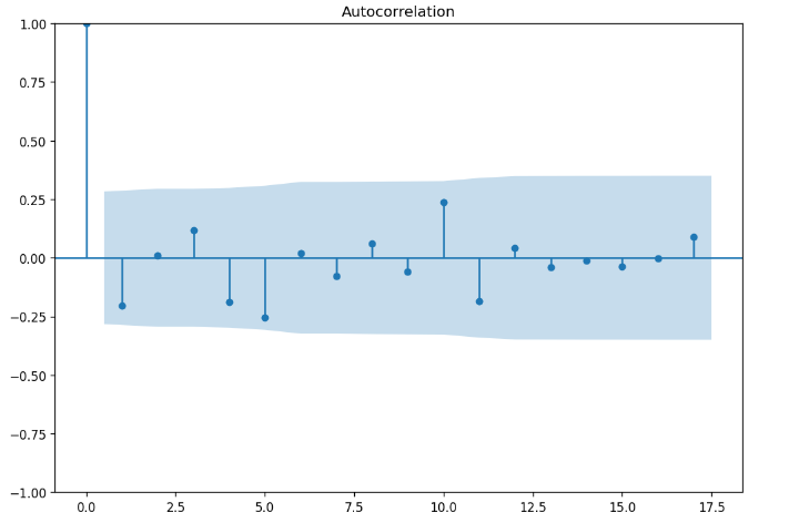
Here, both plots have a horizontal axis that shows the lags, and a vertical axis representing correlation coefficients ranging from -1 to 1 where -1 means perfect negative correlation, 0 means no correlation and 1 means perfect positive correlation.

The blue shaded area represents confidence interval for the correlation coefficients. If the correlation coefficient at a certain lag is outside the confidence interval, it means that the correlation coefficient is statistically significant and not due to chance.

Step 8: Fit the SARIMA Model

Now, fit the SARIMA model using the identified parameters.

SARIMA Parameters: These parameters define the SARIMA model. p, d, and q represent the non-seasonal order, and P, D, Q, and s represent the seasonal order. For example, p is the autoregressive (AR) order, d is the differencing order, and s is the seasonality (in this case, 12 for monthly seasonality).
Fitting the SARIMA Model: Here, a SARIMAX model is created using the defined parameters. The SARIMAX function takes the sales data and the specified order and seasonal_order parameters. The fit method is then called to estimate the model’s coefficients based on the data.

Python

# Define SARIMA parameters
p, d, q = 1, 1, 1
P, D, Q, s = 1, 1, 1, 12  # Assuming monthly seasonality
 
# Fit the SARIMA model
model = SARIMAX(monthly_sales, order=(p, d, q), seasonal_order=(P, D, Q, s))
results = model.fit()
model

Output:

RUNNING THE L-BFGS-B CODE

           * * *

Machine precision = 2.220D-16
 N =            5     M =           10

At X0         0 variables are exactly at the bounds

At iterate    0    f=  4.15152D+00    |proj g|=  2.74080D-01

At iterate    5    f=  4.06571D+00    |proj g|=  1.57031D-02

At iterate   10    f=  4.05982D+00    |proj g|=  4.46554D-03

At iterate   15    f=  4.03337D+00    |proj g|=  1.65496D-02

At iterate   20    f=  4.02336D+00    |proj g|=  3.56570D-02

At iterate   25    f=  4.01887D+00    |proj g|=  6.31166D-04

           * * *

Tit   = total number of iterations
Tnf   = total number of function evaluations
Tnint = total number of segments explored during Cauchy searches
Skip  = number of BFGS updates skipped
Nact  = number of active bounds at final generalized Cauchy point
Projg = norm of the final projected gradient
F     = final function value

           * * *

   N    Tit     Tnf  Tnint  Skip  Nact     Projg        F
    5     28     36      1     0     0   5.795D-06   4.019D+00
  F =   4.0188723995389912     

CONVERGENCE: NORM_OF_PROJECTED_GRADIENT_<=_PGTOL

Step 9: Generate Forecasts

With the model fitted, generate forecasts for future time periods.

In this section of the code, we are using the SARIMA model to forecast future sales values. We specify that we want to forecast the next 12 months by setting forecast_periods to 12.
The results.get_forecast(steps=forecast_periods) function generates the forecast, providing both the predicted mean and a confidence interval for the forecasted values.

Python

# Forecast future values
forecast_periods = 12  # Forecast the next 12 months
forecast = results.get_forecast(steps=forecast_periods)
forecast_mean = forecast.predicted_mean
forecast_ci = forecast.conf_int()
 
# Plot the forecast
plt.figure(figsize=(12, 6))
plt.plot(monthly_sales, label='Observed')
plt.plot(forecast_mean, label='Forecast', color='red')
plt.fill_between(forecast_ci.index, forecast_ci.iloc[:, 0], forecast_ci.iloc[:, 1], color='pink')
plt.title("Sales Forecast")
plt.xlabel("Date")
plt.ylabel("Sales")
plt.legend()
plt.show()

Output:

Forecasting -Geeksforgeeks

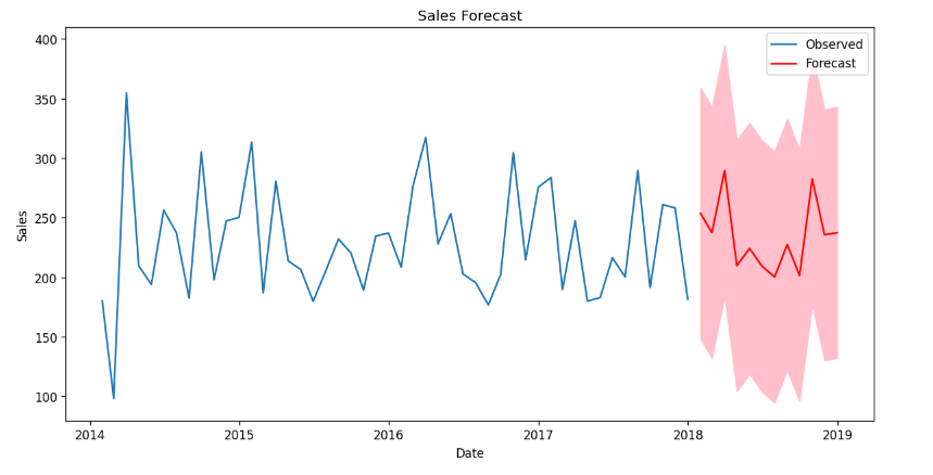
The observed sales data and the forecasted values in red. The pink shaded area represents the confidence interval around the forecast. This visualization helps us understand the expected future sales trends based on our SARIMA model.

Step 10: Evaluate the Model

Let’s evaluate the forecasted sales values by comparing them to the observed sales data using two common metrics for this evaluation: Mean Absolute Error (MAE) and Mean Squared Error (MSE).

MAE (Mean Absolute Error) measures the average absolute difference between the observed and forecasted values. It provides a simple and easily interpretable measure of the model’s accuracy.
MSE (Mean Squared Error) measures the average of the squared differences between the observed and forecasted values. MSE gives more weight to large errors and is sensitive to outliers.
Lower values indicate better performance.

Python

observed = monthly_sales[-forecast_periods:]
mae = mean_absolute_error(observed, forecast_mean)
mse = mean_squared_error(observed, forecast_mean)
print(f'MAE: {mae}')
print(f'MSE: {mse}')

Output:

MAE: 30.815697783063925
MSE: 1302.515608316509

Conclusion

SARIMA models are a potent tool in the realm of time series forecasting. They can capture complex seasonality, long-term trends, and short-term fluctuations in your data. By understanding the components, notation, and best practices of SARIMA modeling, you can make accurate predictions in various domains. So, the next time you encounter time series data, remember the power of SARIMA to unravel its hidden patterns and forecast the future with confidence.

Suggest improvement

Autoregressive (AR) Model for Time Series Forecasting

Share your thoughts in the comments

SARIMA (Seasonal Autoregressive Integrated Moving Average)

Understanding SARIMA

The Components of SARIMA

Seasonal Differencing

The SARIMA Notation

The mathematical representation of SARIMA is as follows:

Use Cases for SARIMA

Implementation of SARIMA for Time Series Forecasting:

Step 1: Import Libraries

Python

Step 2: Load Dataset

Python

Step 3: Extracting monthly sales

Python

Step 5: Plotting the Monhly Sales

Python

Step 6: Check Stationarity

Python

Step 7: Identify Model Parameters

Python

Python

Step 9: Generate Forecasts

Python

Step 10: Evaluate the Model

Python

Conclusion

Please Login to comment...

Similar Reads

What kind of Experience do you want to share?