Standard Test Signals

The standard signals are often used in control systems, signal processing, communication and various engineering applications. These are predefined signals with known characteristics. To clarify standard test signals, their uses and application in the control systems.

In this article, we will be going through standard signals. First of all, we will discuss the basic concepts of signals, and then we will go through 4 standard test signals that are mainly used in control systems followed by definitions, mathematical expressions, representation, properties, real-life examples, and relationships between all 4 standard test signals. At last, we will conclude our article with some interesting FAQs.

What is Signal?

A signal is a physical quantity or a function of one or more independent variables such as Time and Space. It contains or conveys some information. There are many signals in this world which change with respect to Time and Space. Standard test signals are the signals which are used to estimate the performance and characteristics of the system by analyzing the responses of these signals. These signals are applied one by one as input to the system to determine different responses of the system in different cases and then we estimate different characteristics of the system such as Stability, Linearity, Transient response, and Frequency response by analyzing different responses or we can say outputs of the system. In terms of Mathematical representation of signals, these signals are used to represent complex signals.

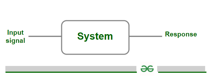
Block diagram of control system

Standard Test Signals

Standard test signals are the signals which are used to check the control systems performance using time response of the output. There are various Standard test signals which are listed below, we will discuss one by one about these signals With their mathematical expressions and graphical representation.

• Step signal
• Ramp signal
• Impulse signal
• Parabolic signal

Step Signal

A Step signal is one of the standard test signal. It is also known as Heaviside’s function or Heaviside’s Step signal. The magnitude of step signal is constant. A Step signal exists only for positive values and zero for negative values. It is denoted by u(t), mathematically u(t) will be constant for t>0 ( i.e., for positive values) and will be zero for t<0 (i.e., for negative values). It represents sudden change in the reference input. It is used to analyze system response to sudden changes in the reference input. It is defined by its magnitude.

There are two types to Step signal , Continuous Step signal and Discrete Step signal.

Continuous Step signal can be defined as the following expression given below-

u(t) = 𝞪 ; for t>=0

0 ; for t<0

Thus the above expression implies that it is a continuous Step signal of magnitude ‘ 𝞪 ‘

For 𝞪 = 1 , This Step signal is called Unit Step signal of magnitude ‘ 1 ‘.

Continuous Unit Step signal can be defined as the following expression given below-

u(t) = 1 ; for t>=0

0 ; for t<0

Graph of Step signal is shown below, fig (i) is graph of Step signal with Magnitude ‘ 𝞪 ‘ and the figure (ii) is graph of Unit Step signal whose magnitude is ‘ 1 ‘

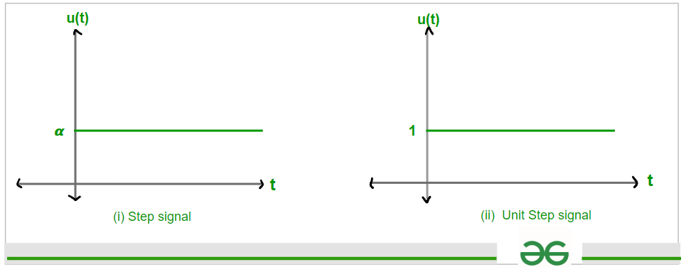
Graph of step signal and unit step signal

Practically, Continuous Unit Step signal can be defined as the following expression given below-

u(t) = 1 ; for t>0

1/2 ; for t=0

0 ; for t<0

At u(0) function is undefined so by using Gibb’s phenomena theory, we will define u(0) as 1/2;

u(0) = { u(0⁺) + u(0^–) }/2

(1+0)/2

1/2 ;

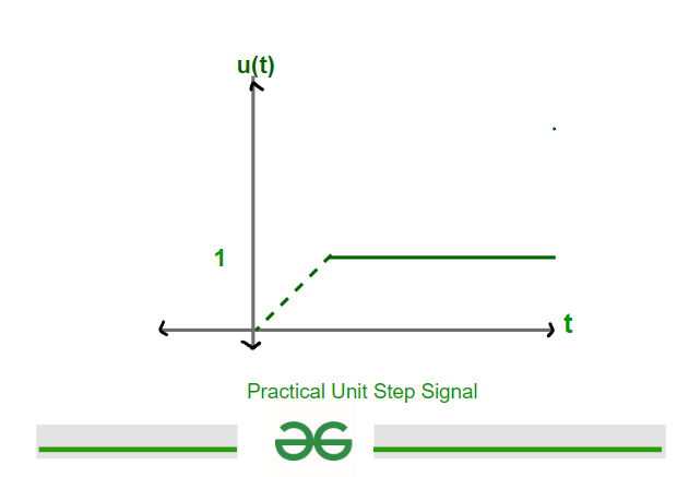
Practical Unit Step signal

Discrete Step signal can be defined as the following expression given below

u[n] = 𝞪 ; for n>0

0 ; for n<0

Where n is an integer.

Thus the above expression implies that it is a Step signal of magnitude ‘ 𝞪 ‘

For 𝞪 = 1 , This Step signal is called Discrete Unit Step signal of magnitude ‘ 1 ‘.

Discrete Unit Step signal can be defined as the following expression given below-

u[n] = 1 ; for n>0

0 ; for n<0

Where n is an integer.

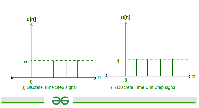
Discrete-Time Step and Unit Step signal

Applications of Step Signals

• System Transitions and Switching Events: Step signals are commonly used to model sudden changes or transitions in systems across various engineering domains.
• Control System Analysis: Step signals are used to analyze the response of control systems to sudden changes in reference inputs or disturbances. By applying step inputs to control systems, we can evaluate system stability, transient response, and performance.
• Process Control and Automation: Step signals are used in process control and automation systems for modeling sudden changes in process parameters, such as flow rates, temperatures, or chemical concentrations.

Advantages of Step Signals

• Simple to Generate : Step signals are simple to generate and understand, making them accessible for both theoretical analysis and practical implementation. Their straightforward nature allows us to easily generate step inputs using simple control mechanisms or software tools.
• System Response to Sudden Changes: Step signals are particularly useful for studying the response of systems to sudden changes or transitions. By applying step inputs to systems, we can observe and analyze how the system reacts to sudden changes in inputs.
• Stability Analysis: We can determine system stability by observing how the system responds to step inputs and By analyzing characteristics such as overshoot, settling time, and steady-state error, which are indicative of stability properties.
• Versatile Applications: Step signals are used in control systems, signal processing, electronics, Motion control and Robotics.

Disadvantages of Step Signals

• Challenges in Generating Perfect Step Signals: Generating perfect step signals in practical systems can be challenging due to limitations in control mechanisms, signal generators, or measurement devices. Imperfections in signal generation, such as transient response, noise, or inaccuracies.
• Discontinuity in Ideal Step Signals: Ideal step signals exhibit discontinuities, transitioning instantaneously from one amplitude to another. Handling such discontinuities in practical systems can be challenging

Ramp Signal

A Ramp signal is one of the standard test signal. It is an increasing function which increases linearly with Time. A Ramp signal exists only for positive values and zero for negative values. It is denoted by r(t), mathematically r(t) will be ‘ t ‘ for t>=0 ( i.e., for positive values of t ) and will be zero for t<0 (i.e., negative values of t ). Ramp signal is used to analyze system response to linearly changing inputs. It is also known as velocity type input. Ramp input is defined by its slope.

There are two types of Ramp signal, Continuous Ramp signal and Discrete Ramp signal.

Continuous Ramp signal can be defined as the following expression given below

r(t) = 𝞪 * t ; for t>=0

0 ; for t<0

Thus the above expression implies that it is a continuous Ramp signal of slope ‘ 𝞪 ‘

For 𝞪 = 1 , This Step signal is called Unit Ramp signal of slope ‘ 1 ‘.

Continuous Unit Ramp Step signal can be defined as the following expression given below-

r(t) = t ; for t>=0

0 ; for t<0

Graph of Ramp signal is shown below, fig (i) is graph of Ramp signal with slope ‘ 𝞪 ‘ and the figure (ii) is graph of Unit Ramp signal whose slope is ‘ 1 ‘

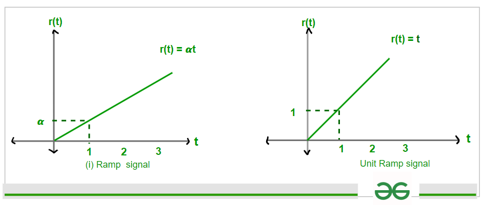
graph of Ramp signal and Unit Ramp signal

Discrete Ramp signal can be defined as the following expression given below

r[n] = 𝞪 * n ; for n>0

0 ; for n<0

Where n is an integer.

Thus the above expression implies that it is a Ramp signal with slope ‘ 𝞪 ‘

For 𝞪 = 1 , This Step signal is called Discrete Unit Ramp signal with slope ‘ 1 ‘.

Discrete Unit Ramp signal can be defined as the following expression given below-

r[n] = n ; for n>0

= 0 ; for n<0

Where n is an integer.

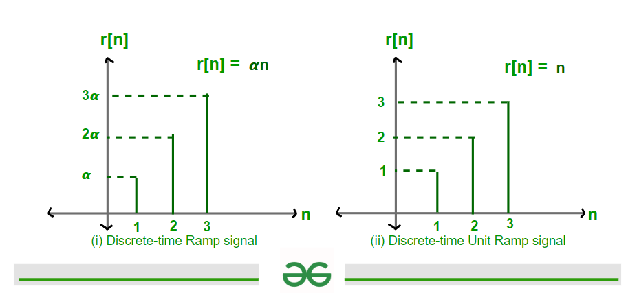
Discrete-Time Ramp and Unit Ramp signal

Applications of Ramp Signals

• Control System Analysis: Ramp signals are to study the response of systems to gradual changes in input. By applying ramp signals as inputs to control systems, we can analyze the system’s response to linearly changing inputs.
• Signal Processing and Filtering: Ramp signals are used in signal processing applications, such as filtering and trend analysis. By convolving signals with ramp functions, we can perform linear trend removal or filtering to extract trends from noisy or fluctuating data.
• Motion Control and Robotics: Ramp signals can be used in motion control systems and robotics. ramp signals are utilized to command smooth and controlled movements of actuators and robotic manipulators.

Advantages of Ramp Signals

• Velocity Profile Representation: Ramp signals are particularly useful for representing velocity profiles in motion control systems.
• Linear Input Analysis: Ramp signals are used to analyze system responses to linearly changing inputs. This allows us to determine how system will react to gradual changes
• Simplified Modeling: Ramp signals offer a straightforward modeling approach for systems that exhibit linear response characteristics. Their simplicity makes them easy to implement and analyze mathematically.
• Versatility in Applications: Ramp signals can be used in different applications across various engineering domains, including motion control, robotics, signal processing, and industrial automation.

Disadvantages of Ramp Signals

• Infinite Energy: Ramp signals have unbounded amplitudes over time, leading to infinite energy. This impracticality arises from the continuous increase or decrease in amplitude, which results in unbounded energy accumulation over time, making it challenging to generate or sustain in real-world systems.
• Unrealistic Modeling: The infinite energy characteristic of ramp signals makes them unrealistic for modeling physical phenomena in the real world. Most physical systems operate within finite energy constraints, and the concept of infinite energy violates the fundamental principles of energy conservation and system stability.
• Complex Analysis: Analyzing the behavior of systems subjected to ramp signals can be complex due to their unbounded nature. Mathematical analysis of systems with infinite energy inputs often involves specialized techniques and considerations, increasing the complexity of system modeling, analysis, and design.

Impulse Signal

An Impulse signal is one of the standard test signal. It is also known as Dirac delta function. An Impulse signal exists only at zero. The magnitude of an Impulse signal is infinity. It is denoted by δ(t), mathematically δ(t) will be infinity at t = 0 and zero for t ≠ 0. An impulse signal is an infinitesimally narrow pulse with unit area and infinite amplitude. It is used to analyze system response to Impulse – like inputs. It gives overall system response. Continuous Impulse signal is defined by its magnitude whereas Discrete Impulse signal is defined by its Amplitude.

There are two types of Impulse signal, Continuous Impulse signal and Discrete Impulse signal.

Continuous Ramp signal can be defined as the following expression given below-

δ(t) = ∞ ; for t = 0

0 ; for t ≠ 0

Area definition of Impulse function :

[Tex] \int_{t = -\infty}^{\infty}\delta(t)dt \space = \space \text{1}[/Tex]

Thus the above expression implies that it is a continuous Unit Impulse signal of Area ‘ 1 ‘

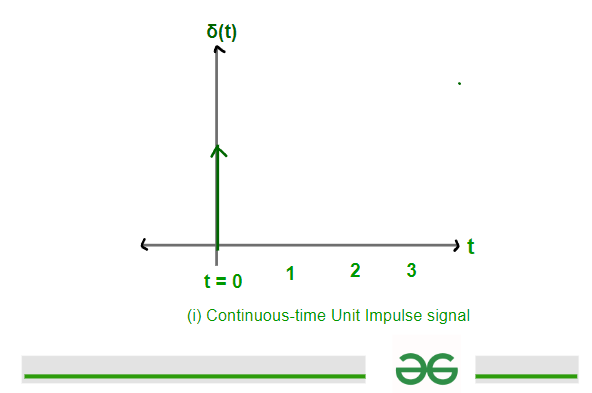
Graph of Continuous-Time Unit Impulse signal

How we generate Continuous impulse signal?

First of all we take a Rectangular ( Gate function ) of area ‘ 1 ‘ unit. Then decrease its width in such a way that its area remain ‘ 1 ‘ unit. When width of Rectangular function tends to zero then height of rectangular function will be of infinite magnitude. It can also be generated by Triangular function with same concept.

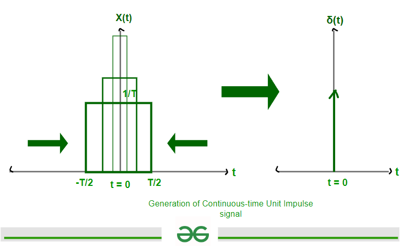
The generation process of Continuous-Time Unit Impulse signal

Properties of Unit Impulse Signal

Given Below are Some of the properties of Unit Impulse Signals

• Area under Unit Impulse function is Unity.

Expression :

[Tex] \int_{-\infty}^{\infty}\delta(t)dt \space = \space \text{1}[/Tex]

• Impulse function is an Even function ( As its graph is symmetric about vertical axis )

Expression :

[Tex] \delta(t) \space = \space \delta(-t)[/Tex]

• Scaling Property of Impulse signal.

Expression :

[Tex] \delta(at) \space = \space \frac{1}{|a|}\delta(t)[/Tex]

• Product property

If X(t) is Continuous at t = 0. Then

1. [Tex] x(t)\delta(t) \space = \space x(0)\delta(t) [/Tex]
2. [Tex]x(t)\delta(t-t_{0}) \space = \space x(t_{0})\delta(t-t_{0}) [/Tex]
3. [Tex] x(t-t_{1})\delta(t-t_{0}) \space = \space x(t_{0}-t_{1})\delta(t-t_{0}) [/Tex]

• Sampling/ Integration property of Impulse function.

1. [Tex]\displaystyle \int_{-\infty}^{\infty}x(t)\delta(t)dt \space = \space \displaystyle\int_{-\infty}^{\infty}x(0)\delta(t)dt \space = \space x(0)\displaystyle\int_{-\infty}^{\infty}\delta(t)dt \space = x(0) [/Tex]
2. [Tex] \displaystyle \int_{-\infty}^{\infty}x(t)\delta(t-t_{0})dt = \displaystyle\int_{-\infty}^{\infty}x(t_{0})\delta(t-t_{0})dt = x(t_{0})\displaystyle\int_{-\infty}^{\infty}\delta(t-t_{0})dt = x(t_{0}) [/Tex]

Discrete-Time Impulse signal can be defined as the following expression given below

δ[n] = 1 ; for n = 0

0 ; for n ≠ 0

Where n is an integer.

Discrete Impulse signal is defined by its magnitude whereas Continuous Impulse signal is defined by area. Discrete Unit Impulse signal is also known as Karnecker’s delta or Unit Sample. δ[n] is not affected by scaling.

Properties of Discrete-Time Unit Impulse signal

• Symmetric Property: Impulse function is an Even function ( As its graph is symmetric about vertical axis ).

Expression :

[Tex] \delta[n] \space = \space \delta[-n][/Tex]

• Scaling Property : Scaling does not affect δ[n].

[Tex] \delta[mn] \space = \space \delta[n] [/Tex]

Proof :

[Tex] \delta[n] \space = \space \begin{cases}\\ 1 , \text{for n = 0}\\ 0, \text{otherwise} \end{cases}[/Tex]

[Tex] \delta[mn] \space = \space \begin{cases}\\ 1 , \text{for mn = 0 \space or n = 0}\\ 0, \text{otherwise} \end{cases}[/Tex]

• Product Property
  

[Tex]x[n]\delta[n] \space = \space x[0]\delta[n] [/Tex]

[Tex] x[n]\delta[n-n_{0}] \space = \space x[n_{0}]\delta[n-n_{0}] [/Tex]

[Tex]x[n-n_{1}]\delta[n-n_{0}] \space = \space x[n_{0} -n_{1}]\delta[n-n_{0}] [/Tex]

• Summation Property

[Tex] \displaystyle\sum_{n=-\infty}^{\infty}x[n]\delta[n] \space = \space \displaystyle\sum_{n=-\infty}^{\infty}x[0]\delta[n] \space = \space x[0] [/Tex]

[Tex]\displaystyle\sum_{n=-\infty}^{\infty}x[n]\delta[n-n_{0}] \space = \space \displaystyle\sum_{n=-\infty}^{\infty}x[n_{0}]\delta[n-n_{0}] \space = \space x[n_{0}] [/Tex]

[Tex] \displaystyle\sum_{n=n_{1}}^{n_{2}}x[n]\delta[n-n_{0}] \space = \space \displaystyle\sum_{n=n_{1}}^{n_{2}}x[n_{0}]\delta[n-n_{0}] \space = \space x[n_{0}], \\ provided \space n_{1} \leq \space n \leq \space n_{2}[/Tex]

Applications of Impulse Signals

• System Analysis : Impulse signals are widely used to analyze the behavior of linear time-invariant (LTI) systems. By applying an impulse signal as input to a system, We can obtain its impulse response, which characterizes the system’s behavior.
• Control System Design: Impulse signals are valuable tools for designing and analyzing control systems. They help to determine the system stability and performance of control systems by evaluating their Impulse response.
• Signal Processing: Impulse signals play a crucial role in signal processing applications such as filtering, convolution, and system identification. For example, in digital signal processing, convolving a signal with an impulse response helps to characterize the system’s behavior and filter out undesired components from the input signal.
• Communication Systems: Impulse signals used in communication systems for channel characterization and modulation schemes. By transmitting impulse-like signals through communication channels, can analyze channel characteristics such as impulse response and frequency response which is crucial for optimizing data transmission and reception.

Advantages of Impulse Signals

• Simplified System Analysis: Impulse signals simplify the analysis of Linear Time-Invariant (LTI) systems. By convolving the impulse response of a system with any input signal, we can obtain the system’s response for that input.
• Universal Response Representation: The impulse response of a system contain its behavior to a unit impulse input, which serves as a basis for understanding its response to any input signal. This universality allows us to analyze and predict the system’s behavior for various input signals without needing to test each input individually.
• Mathematical Simplicity: Impulse signals are easy to represent mathematically. The impulse function, typically denoted as δ(t) or δ[n] in continuous and discrete-time domains, respectively. Its mathematical simplicity facilitates analytical solutions and computations in system analysis and signal processing.
• Time-Invariance Property: Impulse signals exhibit the property of time-invariance, meaning that their response remains consistent over time.

Disadvantages of Impulse Signals

• Idealization vs. Practical Realization: The concept of an impulse signal is mathematically useful for system analysis, practical realization of an ideal impulse signal is not feasible. Ideal impulse signals have zero duration and infinite amplitude, which are physically impossible to generate or measure.
• Physical Constraints: Practical systems and instruments have limitations in terms of bandwidth, resolution, and response time, making it challenging to generate or detect signals with infinitesimally short durations.
• Signal Distortion: Due to limitations in bandwidth and signal processing capabilities, real-world impulse signals are subject to distortion and attenuation.

Parabolic Signal

A Parabolic signal is one of the standard test signal. Parabolic signal is the signal whose magnitude varies as square of time. It is represented by p(t), mathematically p(t) will be t²/2 for t>=0 ( i.e. for positive values) and will be zero for t<0 ( i.e. for negative value ). It is also called acceleration type input. It is used to analyze system response to Non linear inputs.

There are two types to Parabolic signal , Continuous Parabolic signal and Discrete Parabolic signal.

Continuous Parabolic signal can be defined as the following expression given below-

p(t) = t²/2 ; for t>= 0

0 ; for t<0

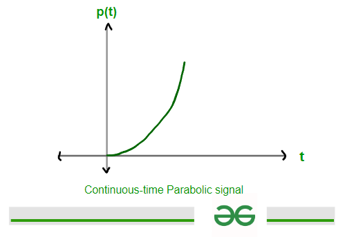
Continuous-Time Parabolic signal

Discrete Parabolic signal can be defined as the following expression given below-

p[n] = n²/2 ; for n>0

= 0 ; for n<0

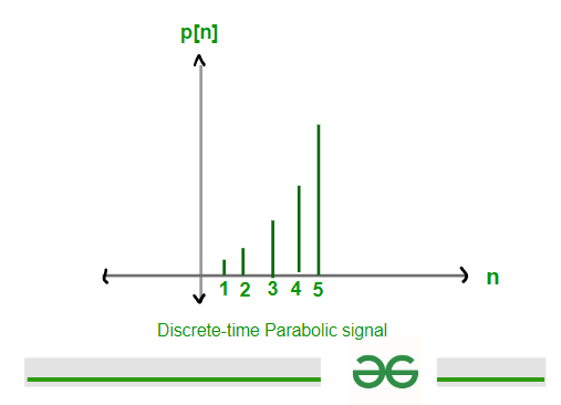
Discrete-Time Parabolic signal

Applications of Parabolic Signals

• Signal processing : Parabolic signals are used in signal processing for analyzing systems with acceleration or deceleration components. It can be used in areas such as audio processing, image processing, and communication systems.
• Control system : parabolic signals help in modeling and analyzing the behavior of dynamic systems, especially those with higher-order dynamics. It can be used in designing controllers for systems with complex dynamics, such as robotics, aerospace systems, and industrial automation.
• Physics and Engineering : Parabolic signals are used in physics and engineering to represent motion, forces, acceleration and energy changes in systems. It can be used in areas like mechanics, fluid dynamics, and structural analysis.

Advantages of Parabolic Signals

• Captures Complex Dynamics: Parabolic signals can represent more complex behaviors compared to simpler signals like ramp signals. It can be used to model systems with acceleration or deceleration, which is essential for understanding real-world phenomena.
• Analysis of Higher-Order Systems: Parabolic signals are useful for analyzing higher-order systems that exhibit non-linear behaviors. It allow to study the response of complex systems to various inputs and disturbances.
• Realistic Modeling: Parabolic signals provide a more realistic modeling approach for systems where acceleration or deceleration is a significant factor, enhancing the fidelity of simulations and predictions.
• Enhanced Control Design: parabolic signals allows for the design of controllers that can handle more complex dynamics, leading to improved system performance and stability.

Disadvantages of Parabolic Signals

• Infinite Energy: Parabolic signals possess infinite energy, which makes them impractical for real-world applications where resources are finite and bounded.
• Complexity in Implementation: Implementing systems that generate or respond to parabolic signals can be challenging due to the need for high-power and complex mechanisms.
• Mathematical Complexity: Analyzing parabolic signals mathematically often requires advanced calculus and differential equations which increases the complexity of modeling and analysis.
• Limited Applicability: simpler signals like steps or ramps are sufficient for modeling and analysis, using of parabolic signals unnecessary and complex.

Relationship Between Signals

Given below are some Relationship between signals :

Relationship Between Step Signal u(t) and Ramp Signal r(t)

X(t) = t for t ⋿ R

X(t) u(t) = t ; for t>= 0

0 ; for t<0

so , t u(t) = r(t)

Graphically, it can be represented as

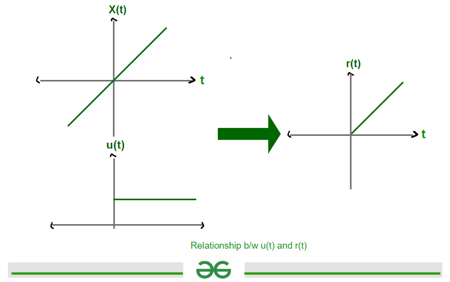
Relationship b/w step and ramp signal

Relationship Between Step Signal u(t) and Impulse Signal δ(t)

Where sudden change or Discontinuity is present at that point Impulse signal will be present.

Expression :

[Tex] \frac{d u(t)}{dt} = \space \delta(t) or \int_{z=-\infty}^{t}\delta(z)dz = \space u(t) [/Tex]

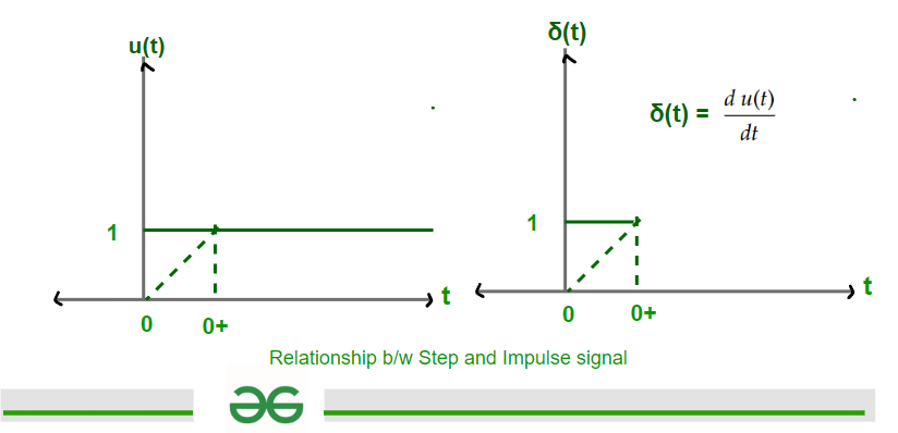
Relationship b/w Step and Impulse signal

Relationship Between Step Signal u(t) and Parabolic signal p(t)

Expression :

[Tex] \frac{d^2 p(t)}{dt} = \space u(t) or p(t) \space = \space \frac{t^2}{2}u(t)[/Tex]

Relationship Between Ramp Signal r(t) and Parabolic signal p(t)

Expression :

[Tex] \frac{d p(t)}{dt} = \space r(t) or \int_{z=-\infty}^{t}r(z)dz = \space p(t) [/Tex]

Standard Test Signals – FAQs

What are the real-life examples of unit step signals?

Real-life examples of step signal are Starting an Electric Motor, Opening a Water Tap, Turning on a Light Switch.

Why we use test signals?

Test signals helps to determine system characteristics such as stability, linearity, frequency response etc.

How can we generate test signals?

Test signals can be generated using a function generator, software or a mathematical algorithm.

What do you understand by Causal, Anti Causal and Non – Causal signal?

Causal signal : A Signal is said to be causal if it is defined for positive values only.

Anti – Causal signal : A Signal is Anti – causal if it is defined for negative values only.

Non – Causal signal : A Signal is said to be Non – Causal if it is defined for both positive and negative values. Also called two sided signal. e.g. – All Periodic signals are Non – Causal signals.