In machine learning, classification is the process of categorizing a given set of data into different categories. In machine learning, to measure the performance of the classification model, we use the confusion matrix. Through this tutorial, understand the significance of the confusion matrix.
What is a Confusion Matrix?
A confusion matrix is a matrix that summarizes the performance of a machine learning model on a set of test data. It is a means of displaying the number of accurate and inaccurate instances based on the model’s predictions. It is often used to measure the performance of classification models, which aim to predict a categorical label for each input instance.
The matrix displays the number of instances produced by the model on the test data.
- True positives (TP): occur when the model accurately predicts a positive data point.
- True negatives (TN): occur when the model accurately predicts a negative data point.
- False positives (FP): occur when the model predicts a positive data point incorrectly.
- False negatives (FN): occur when the model mispredicts a negative data point.
Why do we need a Confusion Matrix?
When assessing a classification model’s performance, a confusion matrix is essential. It offers a thorough analysis of true positive, true negative, false positive, and false negative predictions, facilitating a more profound comprehension of a model’s recall, accuracy, precision, and overall effectiveness in class distinction. When there is an uneven class distribution in a dataset, this matrix is especially helpful in evaluating a model’s performance beyond basic accuracy metrics.
Let’s understand the confusion matrix with the examples:
Confusion Matrix For binary classification
A 2X2 Confusion matrix is shown below for the image recognition having a Dog image or Not Dog image.
| Actual
|
|---|
Dog
| Not Dog
|
|---|
Predicted
| Dog
| True Positive
(TP)
| False Positive
(FP)
|
|---|
Not Dog
| False Negative
(FN)
| True Negative
(TN)
|
|---|
- True Positive (TP): It is the total counts having both predicted and actual values are Dog.
- True Negative (TN): It is the total counts having both predicted and actual values are Not Dog.
- False Positive (FP): It is the total counts having prediction is Dog while actually Not Dog.
- False Negative (FN): It is the total counts having prediction is Not Dog while actually, it is Dog.
Example for binary classification problems
Index
| 1
| 2
| 3
| 4
| 5
| 6
| 7
| 8
| 9
| 10
|
|---|
Actual
| Dog
| Dog
| Dog
| Not Dog
| Dog
| Not Dog
| Dog
| Dog
| Not Dog
| Not Dog
|
|---|
Predicted
| Dog
| Not Dog
| Dog
| Not Dog
| Dog
| Dog
| Dog
| Dog
| Not Dog
| Not Dog
|
|---|
Result
| TP
| FN
| TP
| TN
| TP
| FP
| TP
| TP
| TN
| TN
|
|---|
- Actual Dog Counts = 6
- Actual Not Dog Counts = 4
- True Positive Counts = 5
- False Positive Counts = 1
- True Negative Counts = 3
- False Negative Counts = 1
| Actual
|
|---|
Dog
| Not Dog
|
|---|
Predicted
| Dog
| True Positive
(TP =5)
| False Positive
(FP=1)
|
|---|
Not Dog
| False Negative
(FN =1)
| True Negative
(TN=3)
|
|---|
Metrics based on Confusion Matrix Data
1. Accuracy
Accuracy is used to measure the performance of the model. It is the ratio of Total correct instances to the total instances.

For the above case:
Accuracy = (5+3)/(5+3+1+1) = 8/10 = 0.8
2. Precision
Precision is a measure of how accurate a model’s positive predictions are. It is defined as the ratio of true positive predictions to the total number of positive predictions made by the model.

For the above case:
Precision = 5/(5+1) =5/6 = 0.8333
3. Recall
Recall measures the effectiveness of a classification model in identifying all relevant instances from a dataset. It is the ratio of the number of true positive (TP) instances to the sum of true positive and false negative (FN) instances.

For the above case:
Recall = 5/(5+1) =5/6 = 0.8333
Note: We use precision when we want to minimize false positives, crucial in scenarios like spam email detection where misclassifying a non-spam message as spam is costly. And we use recall when minimizing false negatives is essential, as in medical diagnoses, where identifying all actual positive cases is critical, even if it results in some false positives.
4. F1-Score
F1-score is used to evaluate the overall performance of a classification model. It is the harmonic mean of precision and recall,

For the above case:
F1-Score: = (2* 0.8333* 0.8333)/( 0.8333+ 0.8333) = 0.8333
We balance precision and recall with the F1-score when a trade-off between minimizing false positives and false negatives is necessary, such as in information retrieval systems.
5. Specificity:
Specificity is another important metric in the evaluation of classification models, particularly in binary classification. It measures the ability of a model to correctly identify negative instances. Specificity is also known as the True Negative Rate.

Specificity=3/(1+3)=3/4=0.75
6. Type 1 and Type 2 error
Type 1 error
Type 1 error occurs when the model predicts a positive instance, but it is actually negative. Precision is affected by false positives, as it is the ratio of true positives to the sum of true positives and false positives.

For example, in a courtroom scenario, a Type 1 Error, often referred to as a false positive, occurs when the court mistakenly convicts an individual as guilty when, in truth, they are innocent of the alleged crime. This grave error can have profound consequences, leading to the wrongful punishment of an innocent person who did not commit the offense in question. Preventing Type 1 Errors in legal proceedings is paramount to ensuring that justice is accurately served and innocent individuals are protected from unwarranted harm and punishment.
Type 2 error
Type 2 error occurs when the model fails to predict a positive instance. Recall is directly affected by false negatives, as it is the ratio of true positives to the sum of true positives and false negatives.
In the context of medical testing, a Type 2 Error, often known as a false negative, occurs when a diagnostic test fails to detect the presence of a disease in a patient who genuinely has it. The consequences of such an error are significant, as it may result in a delayed diagnosis and subsequent treatment.

Precision emphasizes minimizing false positives, while recall focuses on minimizing false negatives.
Implementation of Confusion Matrix for Binary classification using Python
Step 1: Import the necessary libraries
Python3
import numpy as np
from sklearn.metrics import confusion_matrix
import seaborn as sns
import matplotlib.pyplot as plt
Step 2: Create the NumPy array for actual and predicted labels
Python3
actual    = np.array(
  ['Dog','Dog','Dog','Not Dog','Dog','Not Dog','Dog','Dog','Not Dog','Not Dog'])
predicted = np.array(
  ['Dog','Not Dog','Dog','Not Dog','Dog','Dog','Dog','Dog','Not Dog','Not Dog'])
Step 3: Compute the confusion matrix
Python3
cm = confusion_matrix(actual,predicted)
Step 4: Plot the confusion matrix with the help of the seaborn heatmap
Python3
sns.heatmap(cm,
            annot=True,
            fmt='g',
            xticklabels=['Dog','Not Dog'],
            yticklabels=['Dog','Not Dog'])
plt.ylabel('Prediction',fontsize=13)
plt.xlabel('Actual',fontsize=13)
plt.title('Confusion Matrix',fontsize=17)
plt.show()
Output:
.png)
Confusion Matrix
Step 5: Classifications Report based on Confusion Metrics
Python3
print(classification_report(actual, predicted))
Output:
              precision    recall  f1-score   support

         Dog       0.83      0.83      0.83         6
     Not Dog       0.75      0.75      0.75         4

    accuracy                           0.80        10
   macro avg       0.79      0.79      0.79        10
weighted avg       0.80      0.80      0.80        10
Confusion Matrix For Multi-class Classification
Now, let’s consider there are three classes. A 3X3 Confusion matrix is shown below for the image having three classes.
Here, TP= True Positive , FP= False Positive , FN= False Negative.
Index
|
1
|
2
|
3
|
4
|
5
|
6
|
7
|
8
|
9
|
10
|
|---|
Actual
| Cat
| Dog
| Horse
| Cat
| Dog
| Cat
| Dog
| Horse
| Horse
| Cat
|
|---|
Predicted
| Cat
| Dog
| Dog
| Cat
| Dog
| Cat
| Dog
| Horse
| Horse
| Dog
|
|---|
Result
| TP
| TP
| FN
| TP
| TP
| TP
| TP
| TP
| TP
| FN
|
|---|
A 3X3 Confusion matrix is shown below for three classes.
| Actual
|
|---|
Cat
| Dog
| Horse
|
|---|
Predicted
| Cat
| TP
| FP
| FP
|
|---|
Dog
| FN
| TP
| FP
|
|---|
Horse
| FN
| FN
| TP
|
For Cat:
- True Positives (TP): 3
- Index 1: True Positive (Cat actual, Cat predicted)
- Index 4: True Positive (Cat actual, Cat predicted)
- Index 6: True Positive (Cat actual, Cat predicted)
- False Negatives (FN): 1
- Index 10: False Negative (Cat actual, Dog predicted)
For Dog:
- True Positives (TP): 5
- Index 2: True Positive (Dog actual, Dog predicted)
- Index 5: True Positive (Dog actual, Dog predicted)
- Index 7: True Positive (Dog actual, Dog predicted)
- Index 10: True Positive (Cat actual, Dog predicted)
- Index 3: False Negative (Horse actual, Dog predicted)
For Horse:
- True Positives (TP): 3
- Index 8: True Positive (Horse actual, Horse predicted)
- Index 9: True Positive (Horse actual, Horse predicted)
- Index 3: False Negative (Horse actual, Dog predicted)
Then, the confusion matrix will be:
| Actual
|
|---|
Cat
| Dog
| Horse
|
|---|
Predicted
| Cat
| TP(3)
| FP(1)
| FP(0)
|
|---|
Dog
| FN(0)
| TP(5)
| FP(1)
|
|---|
Horse
| FN(1)
| FN(1)
| TP(3)
|
Implementation of Confusion Matrix for Binary classification using Python
Step 1: Import the necessary libraries
Python3
import numpy as np
from sklearn.metrics import confusion_matrix, classification_report
import seaborn as sns
import matplotlib.pyplot as plt
Step 2: Create the NumPy array for actual and predicted labels
Python3
actual = np.array(
    ['Cat', 'Dog', 'Horse', 'Cat', 'Dog', 'Cat', 'Dog',  'Horse', 'Horse', 'Cat'])
predicted = np.array(
    ['Cat', 'Dog', 'Dog', 'Cat', 'Dog', 'Cat', 'Dog',  'Horse', 'Horse', 'Dog'])
Step 3: Compute the confusion matrix
Python3
cm = confusion_matrix(actual,predicted)
Step 4: Plot the confusion matrix with the help of the seaborn heatmap
Python3
sns.heatmap(cm,
            annot=True,
            fmt='g',
            xticklabels=['Cat', 'Dog', 'Horse'],
            yticklabels=['Cat', 'Dog', 'Horse'])
plt.ylabel('Prediction', fontsize=13)
plt.xlabel('Actual', fontsize=13)
plt.title('Confusion Matrix', fontsize=17)
plt.show()
Output:
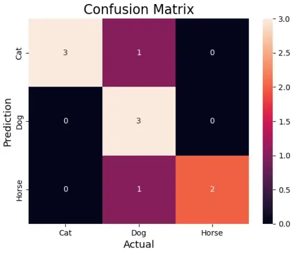
Confusion Matrix for 3 class
Step 5: Classifications Report based on Confusion Metrics
Python3
print(classification_report(actual, predicted))
Output:
              precision    recall  f1-score   support

         Cat       1.00      0.75      0.86         4
         Dog       0.60      1.00      0.75         3
       Horse       1.00      0.67      0.80         3

    accuracy                           0.80        10
   macro avg       0.87      0.81      0.80        10
weighted avg       0.88      0.80      0.81        10
Conclusion
To sum up, the confusion matrix is an essential instrument for evaluating the effectiveness of classification models. Insights into a model’s accuracy, precision, recall, and general efficacy in classifying instances are provided by the thorough analysis of true positive, true negative, false positive, and false negative predictions it offers. The article provided examples to illustrate each metric’s computation and discussed its importance. It also demonstrated how confusion matrices can be implemented in Python for binary and multi-class classification scenarios. Practitioners can make well-informed decisions regarding model performance—particularly when dealing with imbalanced class distributions—by comprehending and applying these metrics.
Frequently Asked Questions (FAQs)
1. How to interpret a confusion matrix?
A confusion matrix summarizes a classification model’s performance, with entries representing true positive, true negative, false positive, and false negative instances, providing insights into model accuracy and errors.
2. What are the advantages of using Confusion matrix?
The confusion matrix provides a comprehensive evaluation of a classification model’s performance, offering insights into true positives, true negatives, false positives, and false negatives, aiding nuanced analysis beyond basic accuracy.
3.What are some examples of confusion matrix applications?
Confusion matrices find applications in various fields, including medical diagnosis (identifying true/false positives/negatives for diseases), fraud detection, sentiment analysis, and image recognition accuracy assessment.
4. What is the confusion matrix diagram?
A confusion matrix diagram visually represents the performance of a classification model. It displays true positive, true negative, false positive, and false negative values in a structured matrix format.
5.What are the three values of the confusion matrix?
The three values of the confusion matrix are true positive (correctly predicted positive instances), true negative (correctly predicted negative instances), and false positive (incorrectly predicted positive instances).
Share your thoughts in the comments
Please Login to comment...