Confidence Interval

In the realm of statistics, precise estimation is paramount to drawing meaningful insights from data. One of the indispensable tools in this pursuit is the confidence interval. Confidence intervals provide a systematic approach to quantifying the uncertainty associated with sample statistics, offering a range within which population parameters are likely to reside. This article seeks to provide a holistic understanding of confidence intervals and empower readers to wield this statistical tool with confidence in their data analyses.

Prerequisites: t-test, z-test

What is Confidence Interval?

Confidence Interval is a range where we are certain that true value exists. The selection of a confidence level for an interval determines the probability that the confidence interval will contain the true parameter value. This range of values is generally used to deal with population-based data, extracting specific, valuable information with a certain amount of confidence, hence the term ‘Confidence Interval’. 

For example:

If we calculate a 95% confidence interval for a population’s average height, and we randomly select a sample of 50 students and calculate their average height to be 165 cm for instance, and the result is a range of 160 to 170 cm, this suggests that if we were to take multiple samples and create confidence intervals in the same manner, we should anticipate that approximately 95% of those intervals would contain the population’s true average height.

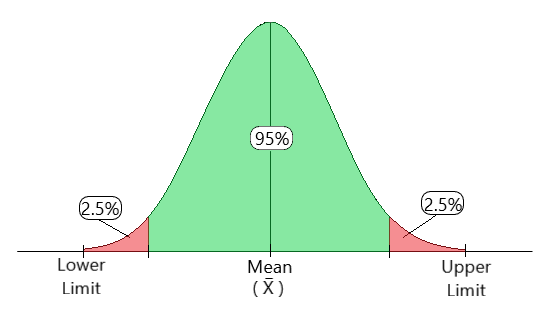
Fig 1: Confidence Interval Illustration

What is Confidence Level?

The confidence level describes the uncertainty associated with a sampling method. 

Suppose we used the same sampling method (say sample mean) to compute a different interval estimate for each sample. Some interval estimates would include the true population parameter, and some would not. 

A 90% confidence level means that we would expect 90% of the interval estimates to include the population parameter. A 95% confidence level means that 95% of the intervals would include the population parameter.

For example:

Let’s suppose you were surveying an average height of men in a particular city. To find that, you set a 95% confidence level and find that the 95% confidence interval is (168,182). That means if you repeated this over and over, 95 percent of the time the height of a man would fall somewhere between 168 cm and 182 cm.

Difference between the Confidence Interval and Confidence Label

Let’s understand the difference between the confidence interval and confidence label.

Aspects	Confidence Interval	Confidence Label
Definition	A confidence interval is a range of values calculated from sample data that is likely to include the true unknown parameter of a population.	The confidence level represents the degree of confidence that the true parameter falls within the calculated confidence interval.
Representation	Numerical range (e.g., [Lower Bound, Upper Bound])	Typically expressed as a percentage (e.g., 95%)
Interpretation	The range within which the true parameter is expected to fall with a certain level of confidence.	The level of confidence in the estimation being made
Example	A 95% confidence interval for the mean height is [65, 70]	We are 95% confident that the true mean height falls within the interval

Steps for Constructing a Confidence Interval

Constructing a confidence interval involves 4 steps:

Step 1: Identify the sample problem. Choose the statistic (like sample mean, etc) that you will use to estimate population parameter.

Clearly define the population parameter you want to estimate and choose an appropriate statistic (e.g., sample mean) to serve as your point estimate.

Step 2: Select a confidence level. (Usually, it is 90%, 95% or 99%)

This reflects the percentage of confidence intervals, derived from random samples, that are expected to contain the true population parameter.

Step 3: Find the margin of error. (Usually given). If not given, use the following formula: –

Finding the critical value

1. Select Significance Level (α): Choose alpha (α), typically 0.05, but adjust as needed based on field standards.
2. Determine Tail Type (One-tailed or Two-tailed): Decide whether a one-tailed or two-tailed interval is appropriate for your analysis. In most cases, a two-tailed interval is used, unless a one-tailed test is specifically required.
3. Adjust Alpha for Tails: For a two-tailed interval, divide the chosen alpha value by two. This adjustment accounts for both the upper and lower tails of the distribution.
4. Consult Critical Value Tables: Refer to critical value tables associated with the relevant statistical distribution (e.g., z-table, t-table) to find the critical value corresponding to the adjusted alpha.

Step 4: Specify the confidence interval. The uncertainty is denoted by the confidence level and the range of the confidence interval is defined by Eq-1.

Use the point estimate, along with the margin of error, to define the interval within which you are reasonably confident the population parameter lies. The confidence interval is typically expressed in the form of “point estimate margin of error.”

                                                                                      ...(1)

A point estimate is a single value that is used to approximate an unknown population parameter. It is calculated from a sample of data and serves as a best guess for the true parameter value. Common examples of point estimates include the sample mean, sample median, and sample proportion.

Types of Confidence Intervals

Some of the common types of Confidence Intervals are:

• Confidence Interval for the Mean of Normally Distributed Data
  A confidence interval for the mean of normally distributed data is often calculated using the t-distribution. This interval provides a range within which the true population mean is likely to fall with a specified level of confidence. The formula incorporates the sample mean, standard deviation, and sample size, and the critical value from the t-distribution table adjusts for smaller sample sizes.
• Confidence Interval for Proportions
  For proportions, a confidence interval estimates the likely range of values for the true population proportion. Typically, the normal approximation or the binomial distribution is used, depending on sample size. The formula involves the sample proportion, standard error, and the critical z-value associated with the chosen confidence level.
• Confidence Interval for Non-Normally Distributed Data
  When dealing with non-normally distributed data or unknown distributions, bootstrap methods offer a flexible approach. Bootstrap confidence intervals involve resampling from the dataset to create multiple samples, allowing for the estimation of the parameter distribution. This technique is particularly useful when assumptions about the data distribution are uncertain or violated.

Calculating Confidence Interval

Calculation of CI requires two statistical parameters. 

• Mean (μ) — Arithmetic mean is the average of numbers. It is defined as the sum of n numbers divided by the count of numbers till n.
  
• Standard deviation (σ) — It is the measure of how spread out the numbers are. It is defined as the summation of squared of the difference between each number and the mean.
  
• Critical Value:

A) Using t-distribution 

We use t-distribution when the sample size n<30. 

Consider the following example. A random sample of 10 UFC fighters was taken and their weights were measured. The mean weight was found to be 240 kg. Construct a 95% confidence interval estimate for the mean weight The sample standard deviation was 25 kg. Find a confidence interval for a sample for the true mean weight of all UFC fighters.

Step 1 – Subtract 1 from your sample size.

This gives the degrees of freedom (df), required in Step-3.

where,

• df = degree of freedom
• n= sample size

Using Eq-5, we get df = 10 – 1 = 9.

Step 2 – Subtract the confidence interval from 1, then divide by two.

This gives the significance level (α), required in Step-3.

• α = Significance level
• CL = Confidence Level

Using Eq-4, we get α = (1 – .95) / 2 = 0.025

Step 3 – Use the values of α and df in the t-distribution table and find the value of t.

(df)/(α)	0.1	0.05	0.025	. .
∞	1.282	1.645	1.960	. .
1	3.078	6.314	12.706	. .
2	1.886	2.920	4.303	. .
:	:	:	:	. .
8	1.397	1.860	2.306	. .
9	1.383	1.833	2.262	. .

Using the values of df and α in the t-distribution table, we get t = 2.262.

Step 4 – Use the t-value obtained in step 3 in the formula given for Confidence Interval with t-distribution. [Eq-6]

where,

• μ = mean
• t = chosen t-value from the table above
• σ = the standard deviation
• n = number of observations

So, putting the values in Eq-6, we get

where,

• Lower Limit = 222.117
• Upper Limit = 257.883

Therefore, we are 95% confident that the true mean weight of the UFC Fighters is between 222.117 and 257.883.

Python implementation

The code uses the ‘scipy.stats’ library module to find the t-value and performs the necessary calculations to obtain the confidence interval. scipy.stats is a subpackage of SciPy, a library in Python for scientific and technical computing. The stats module provides various statistical functions, probability distributions, and statistical tests.

Python3

import scipy.stats as stats
import math

# Given values
sample_mean = 240
sample_std_dev = 25
sample_size = 10
confidence_level = 0.95

# DF
df = sample_size - 1

# Significance level (α)
alpha = (1 - confidence_level) / 2

# t-value from the t-distribution table
t_value = stats.t.ppf(1 - alpha, df)

margin_of_error = t_value * (sample_std_dev / math.sqrt(sample_size))

lower_limit = sample_mean - margin_of_error
upper_limit = sample_mean + margin_of_error

print(f"Confidence Interval: ({lower_limit}, {upper_limit})")

Output:

Confidence Interval: (222.1160773511857, 257.8839226488143)

B) Using a z-distribution

We use z-distribution when the sample size n>30. Z-test is more useful when the standard deviation is known. 

Consider the following example. A random sample of 50 adult females was taken and their RBC count is measured. The sample mean is 4.63 and the standard deviation of RBC count is 0.54. Construct a 95% confidence interval estimate for the true mean RBC count in adult females.

• Step 1 – Find the mean. [Eq-2] (If not already given)
• Step 2 – Find the standard deviation. [Eq-3] (If not already given)
• Step 3 – Determine the z-value for the specified confidence interval.

(some common values in the table given below)

Confidence Interval	z-value
90%	1.645
95%	1.960
99%	2.576

Step 4 – Use the z-value obtained in step 3 in the formula given for Confidence Interval with z-distribution.

where,

• μ = mean
• z = chosen z-value from the table above
• σ = the standard deviation
• n = number of observations

Putting the values in Eq-7, we get

where,

• Lower Limit = 4.480
• Upper Limit = 4.780

Therefore, we are 95% confident that the true mean RBC count of adult females is between 4.480 and 4.780.

Python Implementation

Python3

from scipy import stats
import numpy as np

sample_mean = 4.63
std_dev = 0.54
sample_size = 50
confidence_level = 0.95

# Standard error
standard_error = std_dev / np.sqrt(sample_size)

# z-value for specified confidence interval
z_value = 1.960  # Taken from table for a 95% confidence interval

margin_of_error = z_value * (std_dev / math.sqrt(sample_size))

lower_limit = sample_mean - margin_of_error
upper_limit = sample_mean + margin_of_error

print(f"Confidence Interval: ({lower_limit:.3f}, {upper_limit:.3f})")

Output:

Confidence Interval: (4.480, 4.780)

Factors influencing Confidence Interval

The width of a confidence interval is primarily influenced by three factors:

1. Sample Size (n): Larger sample sizes tend to result in narrower confidence intervals because they provide more precise estimates of the population parameter.
2. Variability in the Data (Standard Deviation or Standard Error): Greater variability in the data leads to wider confidence intervals, as there is more uncertainty in the estimates.
3. Confidence Level (CL): Higher confidence levels, such as 95% or 99%, result in wider intervals. This reflects the trade-off between precision and confidence – higher confidence requires a wider range.

When do you use confidence intervals?

Confidence intervals are an essential tool for determining the range that a population parameter, like a mean or proportion, is most likely to fall into.

1. These intervals give important information about the dependability of study findings and provide a measure of uncertainty around a point estimate.
2. Confidence intervals help researchers express the accuracy of their estimates and make stronger conclusions when working with sample data.
3. Confidence intervals, in essence, give a reasonable range for the true population parameter while acknowledging the inherent variability in data.
4. Confidence intervals are frequently used by researchers in hypothesis testing so they can determine whether a given value falls within the interval and thus influence conclusions about the statistical significance of the data.
5. Whether in medical research, social sciences, or business analytics, the judicious use of confidence intervals enhances the credibility and depth of statistical inferences, fostering a nuanced understanding of the underlying phenomena.

Conclusion

Confidence Interval is one of the foundational concepts of statistics. It tells a statement about the data. Various sampling methods such as mean, median etc. can be used based on the data present. One can also determine what distribution to use when in order to get the best results. For any doubts/queries, comment below.

Frequently Asked Questions (FAQs)

1. What is the 95% confidence interval rule?

The 95% confidence interval rule states that if we repeatedly construct 95% confidence intervals for a population parameter, we can expect 95% of those intervals to contain the true parameter value.

2. What if 95 confidence interval includes 1?

If the 95% confidence interval includes 1, it means that we are not statistically confident in saying that the true parameter value is different from 1. In other words, the data is not strong enough to rule out the possibility that the true parameter value is 1.

3. What is the difference between confidence level and confidence interval?

The confidence level is the probability that the confidence interval contains the true parameter value. The confidence interval is a range of values that is likely to contain the true parameter value.

4. How to find sample size?

The sample size is the number of observations in a sample. The sample size is determined by the desired confidence level, the desired margin of error, and the variability of the data.

5. What is the 5 significance level?

The significance level is the probability of rejecting the null hypothesis when it is actually true. The significance level is typically set at 0.05, which means that we are willing to accept a 5% chance of making a Type I error.