Amazon Product Review Sentiment Analysis using RNN

In this article, we will learn how to use Recurrent Neural Networks for Sentiment Analysis. We will use the Product Reviews dataset which has around 25000 customer reviews. Our end goal will be to give a rating according to the review given.

Sentiment Analysis using RNN

Sentiment Analysis is the process of extracting information from the texts. It involves various steps of Natural Language Processing like, text cleaning, text vectorization, stemming, lemmatization, and many more. We will use the above mentioned steps to finally generate a model that can give rating predictions to the reviews.

Recurrent Neural Networks are a type of neural network which uses previous information to give output. We will use RNN with different setups to get maximum accuracy. Further, we will also use LSTM (Long Short Term Memory) which is an extension to RNN, to further increase the accuracy.

Dataset

We’ve used the dataset i.e. Consumer Reviews of Products. The dataset contains information like reviews and ratings.

Step 1: Importing necessary Libraries

Python3

import pandas as pd
import numpy as np
import matplotlib.pyplot as plt
import re
import seaborn as sns
import nltk
from nltk.corpus import stopwords
from nltk.tokenize import word_tokenize
import tensorflow as tf
from tensorflow.keras.layers import SimpleRNN, LSTM, Dense, Dropout, Embedding,  BatchNormalization
from tensorflow.keras.models import Sequential
from tensorflow.keras.preprocessing.text import Tokenizer
from tensorflow.keras.utils import pad_sequences

import warnings
warnings.filterwarnings('ignore')

Step 2: Loading the dataset

The Amazon dataset contains 25000 customer reviews on Amazon products. Here is how we can load the dataset and get information on it.

Python3

data = pd.read_csv('AmazonReview.csv')

# Printing shape of the dataset
print(data.shape)
# printing columns and rows information
print(data.info())

Output:

(25000, 2)
<class 'pandas.core.frame.DataFrame'>
RangeIndex: 25000 entries, 0 to 24999
Data columns (total 2 columns):
 #   Column     Non-Null Count  Dtype 
---  ------     --------------  ----- 
 0   Review     24999 non-null  object
 1   Sentiment  25000 non-null  int64 
dtypes: int64(1), object(1)
memory usage: 390.8+ KB
None

From the above output, we can see that the dataset is of the shape (25000, 2), which shows that it has 25000 rows and 2 columns.

Step 3: Exploratory Data Analysis

1. As we’ve to just get a sentiment analysis of reviews, so let’s extract useful information from the dataset. Also, let’s look at how many null values are present in this dataset.

Python3

# looking for NULL values
print("Null Values:\n", data.isna().sum())

# dropping null values
data = data.dropna()

# again checking for NULL values
print("Null Values after dropping:\n", data.isna().sum())

Output:

Null Values:
Review       1
Sentiment    0
dtype: int64
Null Values after dropping:
Review       0
Sentiment    0
dtype: int644

Let’s take a look at the number of values of each unique item in the Sentiment column.

Python3

# count of unique values in Sentiment column
data['Sentiment'].value_counts()

1    5000
2    5000
3    5000
4    5000
5    4999
Name: Sentiment, dtype: int64

2. Text Cleaning: In this step, we will clean the ‘reviews.text’ column. We will remove the unwanted HTML tags, brackets, or special characters that may be present in the texts. We will use Regex to clean the text.

Python3

# downloading stopwords from nltk library
nltk.download('stopwords')
stop_words = set(stopwords.words('english'))

# Review text Cleaning
def clean_reviews(text):

    # removing html brackets and other square brackets from the string using regex
    regex = re.compile('<.*?>') # r'<.*?>'
    text = re.sub(regex, '', text)

    # removing special characters like @, #, $, etc
    pattern = re.compile('[^a-zA-z0-9\s]')
    text = re.sub(pattern,'',text)

    # removing numbers
    pattern = re.compile('\d+')
    text = re.sub(pattern,'',text)

    # converting text to lower case
    text = text.lower()

    # Tokenization of words
    text = word_tokenize(text)

    # Stop words removal
    text = [word for word in text if not word in stop_words]

    return text

# using the clean_reviews function on the dataset
data['Review'] = data['Review'].apply(clean_reviews)

4. Tokenization & Text Encoding: In this step, we will use tokenization to first generate the tokens. For this, we will use Tokenizer from the Tensorflow library. And we will encode the text using the same.

We have around 5 unique values in the ‘reviews.rating’ column. So let’s use one-hot encoding to represent each value in the rating as separate columns.

Also, in this step, we have initialized X(input) and y(output) to the model.

Python3

tokenizer = Tokenizer()

# converting all the reviews to list to pass it as a parameter to fit_on_texts
reviews_to_list = data['Review'].tolist()
tokenizer.fit_on_texts(reviews_to_list)

# Generating text sequences
text_sequences = np.array(tokenizer.texts_to_sequences(reviews_to_list))

# one hot encoding
data = pd.get_dummies(data, columns = ['Sentiment'])

# setting maximum words we want in an example
max_words = 500

# Generatin our X (input) to the model
# using pad_sequences and y (output)
X = pad_sequences(text_sequences, maxlen = max_words)
y = data[['Sentiment_1', 'Sentiment_2', 'Sentiment_3', 'Sentiment_4',
       'Sentiment_5']]
print(X.shape, y.shape)

Output:

(24999, 500) (24999, 5)

5. Train-Test Split: In this step, we will split our dataset into training and testing datasets. We will split the dataset into 80-20%, i.e. 80% for the training and 20% for testing.

Python3

# Train Test split
from sklearn.model_selection import train_test_split
X_train, X_test, y_train, y_test = train_test_split(X, y, test_size=0.20, random_state=42)

print(X_train.shape, X_test.shape, y_train.shape, y_test.shape)

Output:

(19999, 500) (5000, 500) (19999, 5) (5000, 5)

Step 4: Model Building, Compiling andLet’s Training

1. Build the Model: In this step, let’s build our model using RNN.

Python3

# Creating a RNN model
rnn = Sequential(name="Simple_RNN")
rnn.add(Embedding(len(tokenizer.word_index)+1,
                        max_words,
                        input_length=max_words))

rnn.add(SimpleRNN(128,activation='relu',return_sequences=True))

rnn.add(SimpleRNN(64,activation='relu',return_sequences=False))

rnn.add(Dense(5, activation='softmax'))

# printing model summary
print(rnn.summary())

Output:

Model: "Simple_RNN"
_________________________________________________________________
 Layer (type)                Output Shape              Param #   
=================================================================
 embedding_1 (Embedding)     (None, 500, 500)          19819500  
                                                                 
 simple_rnn_2 (SimpleRNN)    (None, 500, 128)          80512     
                                                                 
 simple_rnn_3 (SimpleRNN)    (None, 64)                12352     
                                                                 
 dense_1 (Dense)             (None, 5)                 325       
                                                                 
=================================================================
Total params: 19,912,689
Trainable params: 19,912,689
Non-trainable params: 0
_________________________________________________________________
None

2. Compiling the model and Model Evaluation: Let’s compile and train the model we defined in the above step. Then we will see the accuracy of the model on the test dataset.

Python3

# Compiling model
rnn.compile(
    loss="categorical_crossentropy",
    optimizer='adam',
    metrics=['accuracy']
)

# Training the model
history = rnn.fit(X_train, y_train,
                        batch_size=64,
                        epochs=2,
                        verbose=1,
                          validation_data = (X_test, y_test))

# Printing model score on test data
print("Simple_RNN Score---> ", rnn.evaluate(X_test, y_test, verbose=1))

Output:

Epoch 1/2
313/313 [==============================] - 411s 1s/step - loss: 1.4465 - accuracy: 0.3333 
- val_loss: 1.2963 - val_accuracy: 0.4178
Epoch 2/2
313/313 [==============================] - 370s 1s/step - loss: 0.9909 - accuracy: 0.5994 
- val_loss: 1.4120 - val_accuracy: 0.4074

157/157 [==============================] - 13s 83ms/step - loss: 1.4120 - accuracy: 0.4074
Simple_RNN Score--->  [1.4119665622711182, 0.4074000120162964]

Thus we’ve got an accuracy of 40% while using RNN.

LSTM ( Long Short Term Memory)

Let’s use LSTM and see how the model performance is changing. We will simply start with defining the model, compiling and then training. To understand the theoretical aspects of LSTM please visit this article Long Short Term Memory Networks Explanation. 

Python3

model = Sequential(name="LSTM_Model")
model.add(Embedding(len(tokenizer.word_index)+1,
                    max_words,
                    input_length=max_words))

# adding a LSTM layer
model.add(LSTM(150, return_sequences=False))
BatchNormalization()
model.add(Dropout(0.5))

#adding a dense layer with activation function of relu
model.add(Dense(50, activation='relu'))
BatchNormalization()
model.add(Dropout(0.5))

# adding the final output activation with activation function of softmax
model.add(Dense(5, activation='softmax'))

# printing model summary
print(model.summary())

Output:

Model: "LSTM_Model"
_________________________________________________________________
 Layer (type)                Output Shape              Param #   
=================================================================
 embedding_2 (Embedding)     (None, 500, 500)          19819500  
                                                                 
 lstm (LSTM)                 (None, 100)               240400    
                                                                 
 dropout (Dropout)           (None, 100)               0         
                                                                 
 dense_2 (Dense)             (None, 5)                 505       
                                                                 
=================================================================
Total params: 20,060,405
Trainable params: 20,060,405
Non-trainable params: 0
_________________________________________________________________

Python3

# Compiling the model
model.compile(
    loss="categorical_crossentropy",
    optimizer='adam',
    metrics=['accuracy']
)

# Training the GRU model
history = model.fit(X_train, y_train,
                         batch_size=64,
                         epochs=3,
                         verbose=1,
                       validation_data=(X_test, y_test))

# Printing model score on test data
print("LSTM model Score---> ", model.evaluate(X_test, y_test, verbose=1))

Output:

Epoch 1/3
313/313 [==============================] - 59s 176ms/step - loss: 1.3207 - accuracy: 0.4177 
- val_loss: 1.2239 - val_accuracy: 0.4636
Epoch 2/3
313/313 [==============================] - 33s 107ms/step - loss: 1.0189 - accuracy: 0.5793 
- val_loss: 1.2542 - val_accuracy: 0.4542
Epoch 3/3
313/313 [==============================] - 26s 83ms/step - loss: 0.7772 - accuracy: 0.6949 
- val_loss: 1.4089 - val_accuracy: 0.4542

157/157 [==============================] - 2s 10ms/step - loss: 1.4089 - accuracy: 0.4542
LSTM model Score--->  [1.408874273300171, 0.45419999957084656]

Thus we got the final accuracy of 45% using LSTM. Let’s take a look at the classification report of this LSTM model.

Classification Report

Python3

# Plotting the history
metrics = history.history
plt.figure(figsize=(10, 5))

# Plotting training and validation loss
plt.subplot(1, 2, 1)
plt.plot(history.epoch, metrics['loss'], metrics['val_loss'])
plt.legend(['loss', 'val_loss'])
plt.xlabel('Epoch')
plt.ylabel('Loss')

# Plotting training and validation accuracy
plt.subplot(1, 2, 2)
plt.plot(history.epoch, metrics['accuracy'],
         metrics['val_accuracy'])
plt.legend(['accuracy', 'val_accuracy'])
plt.xlabel('Epoch')
plt.ylabel('Accuracy')

Output:

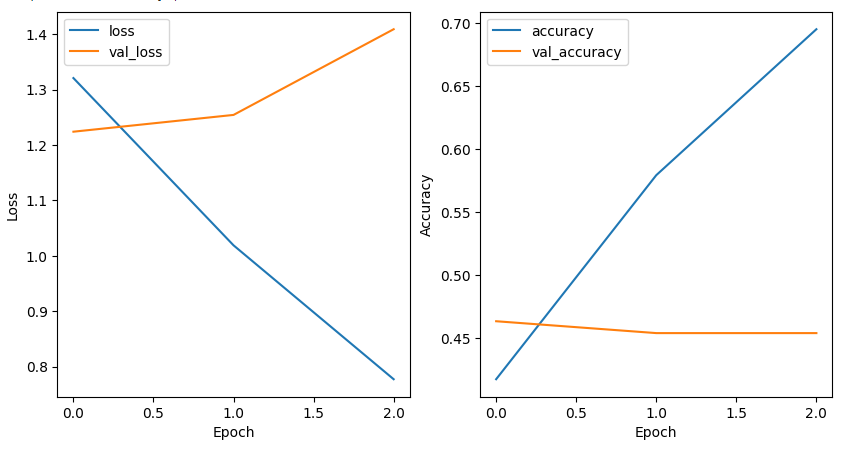
Loss and Accuracy Graph

Python3

# converting y_test tht was one hot encoded to one column fo rconfusion matrix
y_true = np.argmax(y_test.values, axis=1)
y_true.shape

# Confusion matrix
y_pred = np.argmax(model.predict(X_test), axis=1)
cm = tf.math.confusion_matrix(y_true, y_pred)

# Plotting the confusion matrix
plt.figure(figsize=(10, 8))
sns.heatmap(cm, annot=True, fmt='g')
plt.xlabel('Predicted')
plt.ylabel('Actual')
plt.show()

Output:

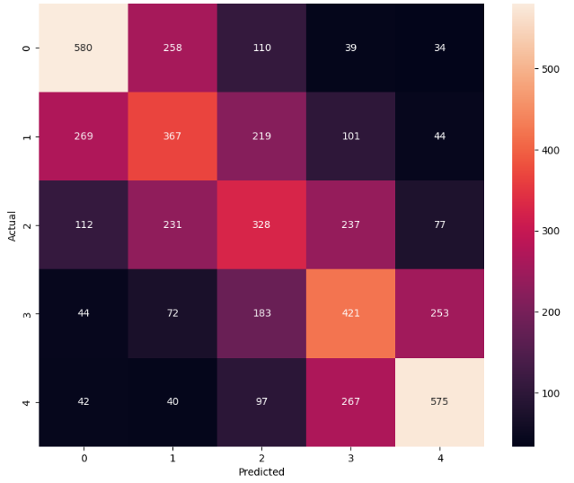
Confusion Matrix

Python3

from sklearn.metrics import classification_report
report = classification_report(y_true, y_pred)
print(report)

Output:

              precision    recall  f1-score   support

           0       0.55      0.57      0.56      1021
           1       0.38      0.37      0.37      1000
           2       0.35      0.33      0.34       985
           3       0.40      0.43      0.41       973
           4       0.58      0.56      0.57      1021

    accuracy                           0.45      5000
   macro avg       0.45      0.45      0.45      5000
weighted avg       0.45      0.45      0.45      5000

Testing the trained model

Let’s take a look at how the model is performing on the text we give in. For this make a custom function in which we will pass out text and it will generate the rating using the model.

Python3

def predict_review_rating(text):
  text_sequences_test = np.array(tokenizer.texts_to_sequences())
  testing = pad_sequences(text_sequences_test, maxlen = max_words)
  y_pred_test = np.argmax(model.predict(testing), axis=1)
  return y_pred_test[0]+1

# Testing
rating1 = predict_review_rating('Worst product')
print("The rating according to the review is: ", rating1)

rating2 = predict_review_rating('Awesome product,  I will recommend this to other users.')
print("The rating according to the review is: ", rating2)

Output:

The rating according to the review is:  1
The rating according to the review is:  5