Emotion Detection Using Convolutional Neural Networks (CNNs)

Emotion detection, also known as facial emotion recognition, is a fascinating field within the realm of artificial intelligence and computer vision. It involves the identification and interpretation of human emotions from facial expressions. Accurate emotion detection has numerous practical applications, including human-computer interaction, customer feedback analysis, and mental health monitoring. Convolutional Neural Networks (CNNs) have emerged as a powerful tool in this domain, revolutionizing the way we understand and process emotional cues from images.

Understanding Emotion Detection

Emotions are a fundamental aspect of human communication and behaviour. They are expressed through facial expressions, body language, and voice tone. While all these cues are important, facial expressions are often the most visible and reliable indicators of emotion. Emotion detection using CNNs focuses primarily on analyzing facial expressions to determine the emotional state of an individual.

Convolutional Neural Network (CNN) Architecture:

Convolutional Neural Networks (CNNs) are a type of deep learning neural network architecture specifically designed for processing grid-like data, such as images and videos. CNNs have revolutionized the field of computer vision and are widely used for various tasks, including image classification, object detection, facial recognition, and image generation. They are particularly effective at capturing spatial hierarchies of features in data.

Below is a simplified architecture of a typical CNN for image classification:

Input Layer:

• The input layer receives the raw image data.
• Images are typically represented as grids of pixels with three color channels (red, green, and blue – RGB).
• The dimensions of the input layer match the dimensions of the input images (e.g., 28x28x1 for a 28×28-pixel image with RGB channels).

Convolutional Layers (Convolutional and Activation):

• Convolutional layers consist of multiple filters (also called kernels).
• Each filter scans over the input image using a sliding window.
• Convolution operation calculates the dot product between the filter and the region of the input.
• Activation functions (e.g., ReLU – Rectified Linear Unit) introduce non-linearity to the network.
• Multiple convolutional layers are used to learn hierarchical features.
• Optional: MaxPooling layers reduce the spatial dimensions (width and height) to reduce computational complexity.

Pooling Layers:

• Pooling layers (e.g., MaxPooling or AveragePooling) reduce the spatial dimensions of feature maps while retaining important information.
• Pooling helps to make the network more robust to variations in the position or size of objects in the input.

Flatten Layer:

• A flatten layer reshapes the output of the previous layers into a 1D vector, allowing it to be input to a dense layer.

Fully Connected Layers:

• After several convolutional and pooling layers, CNNs typically have one or more fully connected layers (also called dense layers).
• Fully connected layers combine high-level features learned from previous layers and make final predictions.
• In classification tasks, these layers output class probabilities.

Loss Function:

• CNNs are trained using a loss function (e.g., categorical cross-entropy for classification) that measures the difference between predicted and actual values.
• The goal during training is to minimize this loss.

Backpropagation and Optimization:

• CNNs are trained using backpropagation and optimization algorithms (e.g., stochastic gradient descent or its variants) to update network parameters (weights and biases) and minimize the loss function.

Model Output:

• The final output is a probability distribution over the classes.
• During training, the model is optimized using a loss function (e.g., categorical cross-entropy) to make its predictions as close as possible to the ground truth labels.

CNNs are designed to automatically learn hierarchical features from input data, making them well-suited for tasks involving structured grid-like data such as images. They have been instrumental in the development of state-of-the-art computer vision applications, including image recognition, object detection, and more. Different CNN architectures, such as VGG, ResNet, and Inception, have been developed to address specific challenges and achieve better performance in various tasks.

Emotion detection using CNNs typically follows these steps:

Build the Emotion Detection Model

Data Collection

A dataset containing labeled facial expressions is collected. Each image in the dataset is labeled with the corresponding emotion (e.g., happy, sad, angry).
Data Set Link: Emotion Detection

Install required packages

!pip install keras
!pip install tensorflow
!pip install --upgrade keras tensorflow
!pip install --upgrade opencv-python

Import required packages

Python3

from keras.models import Sequential
from keras.layers import Conv2D, MaxPooling2D, Dense, Dropout, Flatten
from keras.optimizers import Adam
from keras.preprocessing.image import ImageDataGenerator
from tensorflow.keras.optimizers import Adam
from tensorflow.keras.preprocessing.image import ImageDataGenerator
from tensorflow.keras.optimizers.schedules import ExponentialDecay
import cv2
from keras.models import model_from_json
import numpy as np

Initialize image data generator with rescaling

The rescale parameter is used to normalize the pixel values of the input images by dividing pixel value by 255.

Python3

train_data_gen = ImageDataGenerator(rescale=1./255)
validation_data_gen = ImageDataGenerator(rescale=1./255)

Preprocess all train images

The below code is using the Keras library’s ImageDataGenerator and flow_from_directory functions to create a data generator for training a machine learning model, likely a deep learning model for image classification. Let’s break down the code step by step:

• train_generator = train_data_gen.flow_from_directory(…) – This line creates a data generator named train_generator by calling the flow_from_directory method on an instance of ImageDataGenerator called train_data_gen. The train_data_gen object is presumably configured with various data augmentation and preprocessing settings.
• ‘Train File Path’ – This is the path to the directory containing the training images. The flow_from_directory function will scan this directory and its subdirectories for image files and generate batches of data from them.
• target_size=(48, 48) – This specifies the target size to which the input images will be resized. In this case, the images will be resized to a size of 48×48 pixels. Resizing the images to a consistent size is a common preprocessing step in image-based machine learning tasks.
• batch_size=64 – This sets the batch size for the data generator. It determines how many images will be included in each batch of training data. In this case, each batch will contain 64 images.
• color_mode=”grayscale” – This specifies the color mode for the images. “grayscale” indicates that the images will be converted to grayscale, meaning they will have only one channel (typically representing intensity) instead of the usual three channels (red, green, and blue).
• class_mode=’categorical’ – This indicates the type of labels associated with the images. In this case, it’s set to “categorical,” which means that the labels are one-hot encoded vectors. In other words, each image belongs to one of several categories, and the labels are represented as binary vectors where only one element is “1” to indicate the category to which the image belongs.

Python3

train_generator = train_data_gen.flow_from_directory(
    'Train File Path',
    target_size=(48, 48),
    batch_size=64,
    color_mode="grayscale",
    class_mode='categorical')

Output:

Found 28709 images belonging to 7 classes.

Preprocess all Test Image

Python3

validation_generator = validation_data_gen.flow_from_directory(
        'Test file path',
        target_size=(48, 48),
        batch_size=64,
        color_mode="grayscale",
        class_mode='categorical')

Output:

Found 7178 images belonging to 7 classes.

Create CNN Model Structure

Let’s understand the code to define and compile a Convolutional Neural Network (CNN) model for a specific task, likely emotion recognition from images, step by step:

• emotion_model = Sequential() – This line creates a Sequential model using Keras. A Sequential model is a linear stack of layers, where you can add layers one by one in a sequential manner.
• Convolutional Layers:
  • emotion_model.add(Conv2D(32, kernel_size=(3, 3), activation=’relu’, input_shape=(48, 48, 1)))
  • emotion_model.add(Conv2D(64, kernel_size=(3, 3), activation=’relu’))

These lines add two convolutional layers to the model. Convolutional layers are fundamental in CNNs and are used to detect patterns and features in images. The parameters of each Conv2D layer are as follows: 32 and 64 are the number of filters or kernels in the layers. These filters are responsible for learning different features in the input images.

kernel_size=(3, 3) defines the size of the convolutional kernel or filter.

activation=’relu’ specifies the Rectified Linear Unit (ReLU) activation function, which introduces non-linearity into the model.

input_shape=(48, 48, 1) sets the input shape of the first layer to 48×48 pixels with one channel (grayscale images).

• MaxPooling Layer:
  • emotion_model.add(MaxPooling2D(pool_size=(2, 2)))

This line adds a MaxPooling2D layer after the second convolutional layer. Max pooling reduces the spatial dimensions of the feature maps and helps to retain important features while reducing computational complexity.

• Dropout Layers:
  • emotion_model.add(Dropout(0.25))

These lines add dropout layers with a dropout rate of 25%. Dropout is a regularization technique used to prevent overfitting by randomly deactivating a fraction of neurons during training.

• Additional Convolutional and MaxPooling Layers:
  • emotion_model.add(Conv2D(128, kernel_size=(3, 3), activation=’relu’))
  • emotion_model.add(MaxPooling2D(pool_size=(2, 2)))
  • emotion_model.add(Conv2D(128, kernel_size=(3, 3), activation=’relu’))
  • emotion_model.add(MaxPooling2D(pool_size=(2, 2)))

These lines add two more pairs of convolutional and max-pooling layers, followed by another dropout layer. These layers likely capture higher-level features from the input images.

• Flattening Layer and Dense Layers:
  • emotion_model.add(Flatten())
  • emotion_model.add(Dense(1024, activation=’relu’))
  • emotion_model.add(Dropout(0.5))
  • emotion_model.add(Dense(7, activation=’softmax’))

• Flatten() flattens the output from the previous layers into a 1D vector.

Dense layers are fully connected layers. The first one has 1024 units with ReLU activation, and the second one has 7 units (likely representing the number of emotion classes) with a softmax activation function, which converts the model’s output into class probabilities.

• Learning Rate Schedule:
  • initial_learning_rate = 0.0001
  • lr_schedule = ExponentialDecay(initial_learning_rate, decay_steps=100000, decay_rate=0.96)

This code sets up a learning rate schedule using exponential decay. The learning rate starts at 0.0001 and gradually decreases during training to help the model converge.

• Optimizer:
  • optimizer = Adam(learning_rate=lr_schedule)

The model uses the Adam optimizer with the previously defined learning rate schedule.

• Model Compilation:
  • emotion_model.compile(loss=’categorical_crossentropy’, optimizer=optimizer, metrics=[‘accuracy’])

This line compiles the model, specifying the loss function (‘categorical_crossentropy’ for multi-class classification), the optimizer, and the evaluation metric (‘accuracy’ in this case).

Python3

emotion_model = Sequential()

emotion_model.add(Conv2D(32, kernel_size=(3, 3), activation='relu',
                         input_shape=(48, 48, 1)))
emotion_model.add(Conv2D(64, kernel_size=(3, 3), activation='relu'))
emotion_model.add(MaxPooling2D(pool_size=(2, 2)))
emotion_model.add(Dropout(0.25))

emotion_model.add(Conv2D(128, kernel_size=(3, 3), activation='relu'))
emotion_model.add(MaxPooling2D(pool_size=(2, 2)))
emotion_model.add(Conv2D(128, kernel_size=(3, 3), activation='relu'))
emotion_model.add(MaxPooling2D(pool_size=(2, 2)))
emotion_model.add(Dropout(0.25))

emotion_model.add(Flatten())
emotion_model.add(Dense(1024, activation='relu'))
emotion_model.add(Dropout(0.5))
emotion_model.add(Dense(7, activation='softmax'))

emotion_model.summary()

cv2.ocl.setUseOpenCL(False)

initial_learning_rate = 0.0001
lr_schedule = ExponentialDecay(initial_learning_rate, decay_steps=100000,
                               decay_rate=0.96)

optimizer = Adam(learning_rate=lr_schedule)

emotion_model.compile(loss='categorical_crossentropy', optimizer=optimizer,
                      metrics=['accuracy'])

Output:

Model: "sequential"
_________________________________________________________________
 Layer (type)                Output Shape              Param #   
=================================================================
 conv2d (Conv2D)             (None, 46, 46, 32)        320       
                                                                 
 conv2d_1 (Conv2D)           (None, 44, 44, 64)        18496     
                                                                 
 max_pooling2d (MaxPooling2D  (None, 22, 22, 64)       0         
 )                                                               
                                                                 
 dropout (Dropout)           (None, 22, 22, 64)        0         
                                                                 
 conv2d_2 (Conv2D)           (None, 20, 20, 128)       73856     
                                                                 
 max_pooling2d_1 (MaxPooling  (None, 10, 10, 128)      0         
 2D)                                                             
                                                                 
 conv2d_3 (Conv2D)           (None, 8, 8, 128)         147584    
                                                                 
 max_pooling2d_2 (MaxPooling  (None, 4, 4, 128)        0         
 2D)                                                             
                                                                 
 dropout_1 (Dropout)         (None, 4, 4, 128)         0         
                                                                 
 flatten (Flatten)           (None, 2048)              0         
                                                                 
 dense (Dense)               (None, 1024)              2098176   
                                                                 
 dropout_2 (Dropout)         (None, 1024)              0         
                                                                 
 dense_1 (Dense)             (None, 7)                 7175      
                                                                 
=================================================================
Total params: 2,345,607
Trainable params: 2,345,607
Non-trainable params: 0
_________________________________________________________________

Train The Neural Network Model

The code will train a deep learning model (`emotion_model`) using a data generator (`train_generator`) and validating it using another data generator (`validation_generator`). Let’s break down the code step by step:

• emotion_model_info = emotion_model.fit_generator(…) – This line invokes the fit_generator method on the emotion_model to train the model using data provided by a generator. The training progress and metrics will be stored in the emotion_model_info variable.
• train_generator – This is the data generator used for training the model. It generates batches of training data (input images and their corresponding labels) on the fly from a specified directory of training images.
• steps_per_epoch=28709 // 64 – This parameter specifies how many batches of training data will be processed in each epoch. In this case, it calculates the number of steps needed to process the entire training dataset (with 28,709 samples) in batches of 64 samples each. The double slashes (`//`) indicate integer division, ensuring that the result is an integer.
• epochs=25; This parameter specifies the number of times the entire training dataset will be passed forward and backward through the neural network. In this code, the model will be trained for 25 epochs.
• validation_data=validation_generator – This parameter specifies the data generator used for validation during training. Like the train_generator, the validation_generator generates batches of validation data (usually a separate dataset from the training data) and their labels.
• `validation_steps=7178 // 64` – Similar to steps_per_epoch, this parameter specifies how many batches of validation data will be processed in each validation epoch. It calculates the number of steps needed to process the entire validation dataset (with 7,178 samples) in batches of 64 samples each.

Python3

emotion_model_info = emotion_model.fit_generator(
        train_generator,
        steps_per_epoch=28709 // 64,
        epochs=30,
        validation_data=validation_generator,
        validation_steps=7178 // 64)

Output:

Epoch 1/30
448/448 [==============================] - 292s 648ms/step - loss: 1.8041 - accuracy: 0.2576 - val_loss: 1.7201 - val_accuracy: 0.3280
Epoch 2/30
448/448 [==============================] - 253s 564ms/step - loss: 1.6340 - accuracy: 0.3599 - val_loss: 1.5369 - val_accuracy: 0.4138
Epoch 3/30
448/448 [==============================] - 241s 537ms/step - loss: 1.4511 - accuracy: 0.4430 - val_loss: 1.3922 - val_accuracy: 0.4707
Epoch 5/30
448/448 [==============================] - 250s 558ms/step - loss: 1.3913 - accuracy: 0.4721 - val_loss: 1.3467 - val_accuracy: 0.4887
Epoch 6/30
448/448 [==============================] - 249s 556ms/step - loss: 1.2972 - accuracy: 0.5081 - val_loss: 1.2726 - val_accuracy: 0.5208
Epoch 8/30
448/448 [==============================] - 252s 563ms/step - loss: 1.2629 - accuracy: 0.5213 - val_loss: 1.2393 - val_accuracy: 0.5301
Epoch 9/30
448/448 [==============================] - 245s 547ms/step - loss: 1.2232 - accuracy: 0.5380 - val_loss: 1.2201 - val_accuracy: 0.5342
Epoch 10/30
448/448 [==============================] - 248s 554ms/step - loss: 1.1998 - accuracy: 0.5486 - val_loss: 1.2033 - val_accuracy: 0.5379
Epoch 11/30
448/448 [==============================] - 245s 547ms/step - loss: 1.1670 - accuracy: 0.5610 - val_loss: 1.1784 - val_accuracy: 0.5519
Epoch 12/30
448/448 [==============================] - 253s 565ms/step - loss: 1.1402 - accuracy: 0.5708 - val_loss: 1.1589 - val_accuracy: 0.5611
Epoch 13/30
448/448 [==============================] - 246s 549ms/step - loss: 1.1162 - accuracy: 0.5833 - val_loss: 1.1482 - val_accuracy: 0.5647
Epoch 14/30
448/448 [==============================] - 244s 545ms/step - loss: 1.0864 - accuracy: 0.5924 - val_loss: 1.1396 - val_accuracy: 0.5714
Epoch 15/30
448/448 [==============================] - 244s 545ms/step - loss: 1.0616 - accuracy: 0.6038 - val_loss: 1.1205 - val_accuracy: 0.5781
Epoch 16/30
448/448 [==============================] - 250s 557ms/step - loss: 1.0399 - accuracy: 0.6121 - val_loss: 1.1124 - val_accuracy: 0.5815
Epoch 17/30
448/448 [==============================] - 252s 561ms/step - loss: 1.0124 - accuracy: 0.6255 - val_loss: 1.1126 - val_accuracy: 0.5866
Epoch 18/30
448/448 [==============================] - 241s 537ms/step - loss: 0.9905 - accuracy: 0.6319 - val_loss: 1.0964 - val_accuracy: 0.5901
Epoch 19/30
448/448 [==============================] - 242s 541ms/step - loss: 0.9683 - accuracy: 0.6391 - val_loss: 1.0997 - val_accuracy: 0.5910
Epoch 20/30
448/448 [==============================] - 253s 566ms/step - loss: 0.9435 - accuracy: 0.6494 - val_loss: 1.1042 - val_accuracy: 0.5855
Epoch 21/30
448/448 [==============================] - 246s 548ms/step - loss: 0.9255 - accuracy: 0.6573 - val_loss: 1.0873 - val_accuracy: 0.5938
Epoch 22/30
448/448 [==============================] - 250s 559ms/step - loss: 0.9014 - accuracy: 0.6696 - val_loss: 1.0791 - val_accuracy: 0.6037
Epoch 23/30
448/448 [==============================] - 253s 564ms/step - loss: 0.8751 - accuracy: 0.6802 - val_loss: 1.0696 - val_accuracy: 0.6037
Epoch 24/30
448/448 [==============================] - 248s 553ms/step - loss: 0.8585 - accuracy: 0.6855 - val_loss: 1.0705 - val_accuracy: 0.6059
Epoch 25/30
448/448 [==============================] - 242s 539ms/step - loss: 0.8325 - accuracy: 0.6920 - val_loss: 1.0755 - val_accuracy: 0.6007
Epoch 26/30
448/448 [==============================] - 250s 559ms/step - loss: 0.8117 - accuracy: 0.7038 - val_loss: 1.0733 - val_accuracy: 0.6095
Epoch 27/30
448/448 [==============================] - 242s 541ms/step - loss: 0.7852 - accuracy: 0.7107 - val_loss: 1.0671 - val_accuracy: 0.6115
Epoch 28/30
448/448 [==============================] - 242s 540ms/step - loss: 0.7645 - accuracy: 0.7199 - val_loss: 1.0661 - val_accuracy: 0.6144
Epoch 29/30
448/448 [==============================] - 252s 562ms/step - loss: 0.7386 - accuracy: 0.7301 - val_loss: 1.0779 - val_accuracy: 0.6124
Epoch 30/30
448/448 [==============================] - 244s 545ms/step - loss: 0.7135 - accuracy: 0.7423 - val_loss: 1.0744 - val_accuracy: 0.6110

• “Epoch 1/30”: This line indicates that the training process is in its first epoch out of a total of 30 epochs. An epoch is one complete pass through the entire training dataset.
• “448/448 [==============================]”: This line provides information about the progress within the current epoch. It typically includes two numbers: the current batch number and the total number of batches in the epoch. In this case, there are 448 batches in the training dataset.
• “[==============================]”: The equal signs in square brackets represent a progress bar that fills as the training progresses. It gives you a visual indication of how far along the current epoch is.
• “- loss: 1.8041”: This line shows the current value of the loss function for the training data. The loss function measures the error between the predicted values and the actual target values. In this case, the loss is 1.8082 for the current batch.
• “- accuracy: 0.2576”: This line shows the current accuracy on the training data. The accuracy is a measure of how well the model is performing on the training dataset. In this case, the accuracy is 0.2576 for the current batch.
• “val_loss: 1.7201”: This line shows the value of the loss function on the validation dataset. The validation loss measures how well the model is performing on data it has not seen during training.
• “val_accuracy: 0.3280”: This line shows the accuracy on the validation dataset. It’s a measure of how well the model generalizes to new, unseen data.

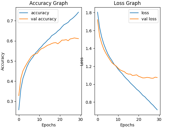
Throughout the output, you can see that the model is being trained for 30 epochs. The loss is gradually decreasing, and the accuracy is increasing on both the training and validation datasets. This suggests that the model is learning and improving its performance over time. The goal of training is to minimize the loss and maximize the accuracy on the validation dataset.

The training process involves adjusting the model’s weights and biases iteratively to improve its ability to make predictions. Typically, as the number of epochs increases, the model’s performance on the training dataset improves, but it’s essential to monitor the validation metrics to ensure that the model is not overfitting (i.e., performing well on training data but not generalizing to new data).

Accuracy and Loss Evaluation

Python

emotion_model.evaluate(validation_generator)

Output:

113/113 [==============================] - 14s 124ms\step  - loss: 1.0744 - accuracy: 0.6110
[1.0743528604507446, 0.6110337376594543]

Visualizing Accuracy and Loss

The code is used to extract training and validation, accuracy and loss values from keras model’s history object.

Python3

accuracy = emotion_model_info.history['accuracy']
val_accuracy = emotion_model_info.history['val_accuracy']
loss = emotion_model_info.history['loss']
val_loss = emotion_model_info.history['val_loss']

Subplot for Accuracy and loss Graph:

Python3

import matplotlib.pyplot as plt

# Accuracy graph
plt.subplot(1, 2, 1)
plt.plot(accuracy, label='accuracy')
plt.plot(val_accuracy, label='val accuracy')
plt.title('Accuracy Graph')
plt.xlabel('Epochs')
plt.ylabel('Accuracy')
plt.legend()

# loss graph
plt.subplot(1, 2, 2)
plt.plot(loss, label='loss')
plt.plot(val_loss, label='val loss')
plt.title('Loss Graph')
plt.xlabel('Epochs')
plt.ylabel('Loss')
plt.legend()

plt.show()

Output:

Save Model Structure In Json File

The code snippet will be responsible for saving a trained deep learning model (in this case, named emotion_model) in two different files: one for the model architecture in JSON format and another for the model’s trained weights in an HDF5 (.h5) format. Let’s break down and understand the code step by step:

• model_json = emotion_model.to_json() – This line converts the architecture and configuration of the emotion_model to a JSON (JavaScript Object Notation) format. The model’s architecture includes information about the layers, their configurations, and how they are connected. This JSON representation is a text-based format and can be easily saved to a file.
• with open(“emotion_model.json”, “w”) as json_file – This code opens a file named “emotion_model.json” in write mode (`”w”`), and it uses a context manager (`with` statement) to ensure that the file is properly closed when the operations inside the block are done.
• json_file.write(model_json) – This line writes the JSON representation of the model’s architecture (model_json) into the “emotion_model.json” file. After this step, you will have a file containing the model’s architecture.
• emotion_model.save_weights(’emotion_model.h5′) – This line saves the trained weights of the emotion_model to a separate file named “emotion_model.h5” The .h5 format is a common choice for storing model weights in deep learning because it supports saving complex data structures efficiently.

Python3

model_json = emotion_model.to_json()
with open("emotion_model.json", "w") as json_file:
    json_file.write(model_json)

# save trained model weight in .h5 file
emotion_model.save_weights('emotion_model.h5')

Live Predictions

Create a Dictionary For Different Type Of Emotion

The code creates a dictionary with integers keys and string values representing different types of emotions.

Python3

emotion_dict = {0: "Angry", 1: "Disgusted", 2: "Fearful",
                3: "Happy", 4: "Neutral", 5: "Sad", 6: "Surprised"}

Load Json and Create Model

The code will read a json file containing a Keras model’s architecture and creates a new model instances from it.

Python3

json_file = open('emotion_model.json', 'r')
loaded_model_json = json_file.read()
json_file.close()
emotion_model = model_from_json(loaded_model_json)

Validation and Testing

The below code is an implementation of real-time emotion detection using a webcam or camera feed. It continuously captures frames from the camera, detects faces in each frame, preprocesses the detected faces, predicts the emotions associated with those faces using a pre-trained deep learning model, and then draws bounding boxes around the faces with emotion labels. Let’s break down the code step by step:

• while True – This initiates an infinite loop, which continuously captures frames from the camera and processes them until the loop is manually terminated.
• ret, frame = cap.read() – This line reads a frame from the camera using the `cap` object (assumed to be a VideoCapture object). It returns two values: `ret`, a Boolean indicating whether the frame was successfully read, and `frame`, the captured image.
• frame = cv2.resize(frame, (1280, 720)) – This line resizes the captured frame to a width of 1280 pixels and a height of 720 pixels. Resizing the frame is often done to standardize the input size for processing.
• if not ret – This condition checks if the frame was not successfully read. If it wasn’t, it breaks out of the loop, effectively ending the program.
• face_detector = cv2.CascadeClassifier(‘haarcascades/haarcascade_frontalface_default.xml’) – This line initializes a face detection classifier using a Haar Cascade classifier. It uses the XML file ‘haarcascade_frontalface_default.xml’ to detect faces in the frame.
  • Download Link(haarcascade_frontalface_default.xml): https://github.com/opencv/opencv/blob/4.x/data/haarcascades/haarcascade_frontalface_default.xml
• gray_frame = cv2.cvtColor(frame, cv2.COLOR_BGR2GRAY) – This converts the resized frame from color (BGR) to grayscale. Many face detection algorithms work better with grayscale images.
• num_faces = face_detector.detectMultiScale(gray_frame, scaleFactor=1.3, minNeighbors=5) – This line detects faces in the grayscale frame using the Haar Cascade classifier. It returns a list of rectangles, where each rectangle represents a detected face. Parameters like `scaleFactor` and `minNeighbors` control the sensitivity and accuracy of face detection.
• Loop over detected faces – The code then enters a loop to process each detected face one by one.
  • `cv2.rectangle(frame, (x, y-50), (x+w, y+h+10), (0, 255, 0), 4)` draws a green bounding box around the detected face on the original frame.
  • `roi_gray_frame` is a region of interest (ROI) that corresponds to the detected face in the grayscale frame.
  • `cropped_img` preprocesses the ROI by resizing it to 48×48 pixels and converting it to a 3D numpy array.
  • `emotion_model.predict(cropped_img)` predicts the emotion associated with the preprocessed face using a pre-trained deep learning model (`emotion_model`).

The predicted emotion label is added to the frame using `cv2.putText`, and it’s positioned just above the bounding box.

• cv2.imshow(‘Emotion Detection’, frame) – This displays the frame with bounding boxes and emotion labels in a window with the title ‘Emotion Detection.’
• if cv2.waitKey(1) & 0xFF == ord(‘q’) – This checks if the ‘q’ key is pressed. If ‘q’ is pressed, it breaks out of the loop, ending the program.
• cap.release()` and `cv2.destroyAllWindows() – These lines release the camera or video feed and close all OpenCV windows when the program is terminated.

Python3

cap = cv2.VideoCapture(0)
while True:
    # Find haar cascade to draw bounding box around face
    ret, frame = cap.read()
    frame = cv2.resize(frame, (1280, 720))
    if not ret:
        print(ret)
    # Create a face detector
    face_detector = cv2.CascadeClassifier(cv2.data.haarcascades + 'haarcascade_frontalface_default.xml')

    gray_frame = cv2.cvtColor(frame, cv2.COLOR_BGR2GRAY)

    # detect faces available on camera
    num_faces = face_detector.detectMultiScale(gray_frame,
                                               scaleFactor=1.3, minNeighbors=5)

    # take each face available on the camera and Preprocess it
    for (x, y, w, h) in num_faces:
      cv2.rectangle(frame, (x, y-50), (x+w, y+h+10), (0, 255, 0), 4)
        roi_gray_frame = gray_frame[y:y + h, x:x + w]
        cropped_img = np.expand_dims(np.expand_dims(cv2.resize(roi_gray_frame,
                                                               (48, 48)), -1), 0)

        # predict the emotions
        emotion_prediction = emotion_model.predict(cropped_img)
        maxindex = int(np.argmax(emotion_prediction))
        cv2.putText(frame, emotion_dict[maxindex], (x+5, y-20),
                    cv2.FONT_HERSHEY_SIMPLEX, 1, (0, 0, 255), 2, cv2.LINE_AA)

    cv2.imshow('Emotion Detection', frame)
    if cv2.waitKey(1) & 0xFF == ord('q'):
        break

cap.release()
cv2.destroyAllWindows()

Output:

Output Of The Model

Conclusion

Emotion detection using Convolutional Neural Networks has the potential to revolutionize how we interact with technology and understand human emotions. As the field continues to advance, we can expect to see more emotionally intelligent applications across various domains, enhancing user experiences and improving our ability to empathize and connect with one another. With continued research and development, CNN-based emotion detection systems will play a pivotal role in shaping the future of artificial intelligence and human-computer interaction.