Generalized Additive Models Using R

A versatile and effective statistical modeling method called a generalized additive model (GAM) expands the scope of linear regression to include non-linear interactions between variables. Generalized additive models (GAMs) are very helpful when analyzing complicated data that displays non-linear patterns, such as time series, and spatial data, or when the connections between predictors and the response variable are difficult to describe by straightforward linear functions. We’ll look at the basics of GAMs in this guide and show you how to use them in the R Programming Language.

Generalized Additive Models (GAMs)

Traditional linear regression models assume a linear relationship between predictors and the response variable. However, many real-world phenomena exhibit non-linear, complex relationships. GAMs address this limitation by allowing for flexible modeling of these relationships through the use of smoothing functions. This makes GAMs a valuable tool for capturing patterns in data that linear models might miss.

A generalized additive model (GAM) is a generalized linear model in which the linear response variable depends linearly on unknown smooth functions of some predictor variables, and interest focuses on inference about these smooth functions.

Basic Components of a GAM

• Linear Predictors: GAMs include linear predictors, similar to traditional linear regression modelling, but they also incorporate additional components.
• Smooth Functions: GAMs employ smooth functions to capture non-linear relationships. These functions are typically spline functions or other types of smooth curves.
• Link Function: Like generalized linear models (GLMs), GAMs use a link function to relate the expected value of the response variable to the linear predictor.
• Additive Structure: GAMs are additive models, meaning that the contribution of each smooth function is additive, allowing for the modelling of complex relationships as a sum of simpler components.

Understanding GAMs

Its been known that any multivariate function could be represented as sums and compositions of univariate functions.

But they require highly complicated functions and thus are not suitable for modelling approaches. Therefore, GAMs dropped the outer sum and made sure the function belongs to simpler class.

where ???? is a smooth monotonic function. Writing g for the inverse of ????, this is traditionally written as

When this function is approximating the expectation of some observed quantity, it could be written as

This is the standard formulation of a GAM.

Generalized Additive Model on mtcars dataset

Pre-Requisites

To work with GAMs in R, you’ll need to install and load the mgcv package, which is a widely-used package for fitting GAMs along with ggplot2- used for data visualisation. You can install them using the following command:

install.packages('mgcv')
install.packages('ggplot2')

Loading Packages

R

# Load required packages
library(mgcv)
library(ggplot2)

Load the dataset

R

# Load the mtcars dataset
data(mtcars)
head(mtcars)

Output:

                   mpg cyl disp  hp drat    wt  qsec vs am gear carb
Mazda RX4         21.0   6  160 110 3.90 2.620 16.46  0  1    4    4
Mazda RX4 Wag     21.0   6  160 110 3.90 2.875 17.02  0  1    4    4
Datsun 710        22.8   4  108  93 3.85 2.320 18.61  1  1    4    1
Hornet 4 Drive    21.4   6  258 110 3.08 3.215 19.44  1  0    3    1
Hornet Sportabout 18.7   8  360 175 3.15 3.440 17.02  0  0    3    2
Valiant           18.1   6  225 105 2.76 3.460 20.22  1  0    3    1

Building Model

R

# Fit a GAM to model the relationship between mpg and hp
gam_model <- gam(mpg ~ s(hp), data = mtcars)

# Summary of the GAM
summary(gam_model)

Output:

Family: gaussian 
Link function: identity 
Formula:
mpg ~ s(hp)
Parametric coefficients:
            Estimate Std. Error t value Pr(>|t|)    
(Intercept)  20.0906     0.5487   36.62   <2e-16 ***
---
Signif. codes:  0 ‘***’ 0.001 ‘**’ 0.01 ‘*’ 0.05 ‘.’ 0.1 ‘ ’ 1
Approximate significance of smooth terms:
        edf Ref.df     F  p-value    
s(hp) 2.618  3.263 26.26 2.29e-10 ***
---
Signif. codes:  0 ‘***’ 0.001 ‘**’ 0.01 ‘*’ 0.05 ‘.’ 0.1 ‘ ’ 1
R-sq.(adj) =  0.735   Deviance explained = 75.7%
GCV = 10.862  Scale est. = 9.6335    n = 32

First we install and load the necessary R packages mgcv and ggplot2. The mgcv package is used for fitting Generalized Additive Models (GAMs), and ggplot2 is used for data visualization. We also load the built-in mtcars dataset, which contains information about various car models, including their miles per gallon (mpg) and horsepower (hp).

• Generalized Additive Model (GAM) is fitted using the gam function from the mgcv package. The model is specified with the formula mpg ~ s(hp), which means we want to model the relationship between miles per gallon (mpg) and the smoothed term of horsepower (s(hp)). The data for this modeling is taken from the mtcars dataset.
• The summary includes important information such as estimated coefficients, degrees of freedom, p-values for the smooth term, and other statistics related to the model fit.

Visualize the results

R

# Generate the random hp dataset for predictions
new_data <- data.frame(hp = seq(min(mtcars$hp), max(mtcars$hp),
                                length.out = 100))
predictions <- predict(gam_model, newdata = new_data, type = "response",
                       se.fit = TRUE)

# Plot the data and the GAM fit
ggplot() +
  geom_point(data = mtcars, aes(x = hp, y = mpg)) +
  geom_line(data = data.frame(hp = new_data$hp, mpg = predictions$fit),
            aes(x = hp, y = mpg), color = "blue", size = 1) +
  geom_ribbon(data = data.frame(hp = new_data$hp, fit = predictions$fit,
                                se = predictions$se.fit), aes(x = hp,
                                ymin = fit - 1.96 * se,
                                ymax = fit + 1.96 * se), alpha = 0.3) +
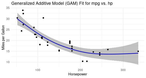
  labs(title = "Generalized Additive Model (GAM) Fit for mpg vs. hp",
       x = "Horsepower", y = "Miles per Gallon") +
  theme_minimal()

Output:

Generalized Additive Models Using R

First a new data frame new_data is created. It includes a sequence of values for horsepower (hp) spanning the range of the hp values in the mtcars dataset. This new data is used to make predictions using the fitted GAM model. The predict function is used to obtain these predictions. The type = “response” argument ensures we get the predicted values on the original scale (miles per gallon) rather than on the link scale. The se.fit = TRUE argument also calculates standard errors for the predictions.

• the ggplot2 package to create a data visualization. The ggplot() function initializes a new plot. We then add the following layers to the plot:
• geom_point: Adds the original data points from the mtcars dataset, with x representing hp and y representing mpg.
• geom_line: Adds a smooth curve representing the GAM fit. The predictions$fit values are plotted against new_data$hp.
• geom_ribbon: Adds a shaded area representing the 95% confidence interval around the GAM fit. This interval is calculated using the standard errors (predictions$se.fit) and is shaded in a translucent blue.
• labs: Sets the title and axis labels for the plot.
• theme_minimal: Applies a minimalistic theme to the plot for a cleaner appearance.
• The resulting plot displays the data points, the smooth GAM curve, and the confidence interval, providing a visual representation of the relationship between miles per gallon and horsepower in the mtcars dataset.

Finally, we create a visualization of the fitted GAM model and the original data. The plot(gam_model) function generates a plot that shows the smooth curve representing the relationship between age and tree height, as well as the individual data points.

Conclusion

In conclusion, Generalized Additive Models (GAMs) offer a flexible and powerful approach to modeling complex relationships in data. This guide provides an overview of GAMs, their implementation in R, interpretation, model evaluation, and advanced topics. To deepen your understanding and expertise in GAMs, consider further reading and hands-on practice with real-world datasets.