Markov Models. Using R

Markov models are powerful tools used in various fields such as finance, biology, and natural language processing. They are particularly useful for modeling systems where the next state depends only on the current state and not on the sequence of events that preceded it. In this article, we will delve into the concept of Markov models and demonstrate how to implement them using the R programming language.

What is a Markov Model?

A Markov Model is a way of describing how something changes over time. It works by saying that the chance of something happening next only depends on what’s happening right now, not on how it got to this point. Imagine a game where you move from one square to another on a board. The next square you land on only depends on the current square you’re on, not how you moved there before. Markov Models are used to understand and predict these kinds of situations.

Types of Markov models

Two commonly applied types of Markov model are used when the system being represented is autonomous — that is, when the system isn’t influenced by an external agent. These are as follows:

1.Markov Chains

Markov models are often visualized as Markov chains, where each state is represented as a node, and the transitions between states are depicted as directed edges. The probability of transitioning from one state to another is associated with the corresponding edge.

Imagine we have three types of weather: sunny, cloudy, and rainy. We want to predict the weather for the next day based on the current day. We can use a Markov Chain to represent this.

Here’s how we visualize it:

• States: Sunny, Cloudy, Rainy (represented as nodes)
• Transitions: Arrows between the states represent the likelihood of moving from one weather type to another.

Now, let’s consider the probabilities associated with each transition:

• If it’s sunny today, there’s a 70% chance it will be sunny again tomorrow (arrow pointing to sunny).
• If it’s sunny today, there’s a 20% chance it will be cloudy tomorrow (arrow pointing to cloudy).
• If it’s sunny today, there’s a 10% chance it will be rainy tomorrow (arrow pointing to rainy).
• This pattern continues for each weather type, indicating the probabilities of transitioning to other states.

So, a Markov Chain for this weather model visually shows how likely it is to move from one weather state to another. It simplifies the prediction process by focusing only on the current state and the associated probabilities for transitioning to the next state.

2.Hidden Markov Models (HMMs)

Suitable for systems with unobservable states, HMMs include observations and observation likelihoods for each state. They find application in thermodynamics, finance, and pattern recognition.

• In speech recognition, words spoken form the observable states, but the actual phonemes (basic sound units) producing those words are hidden. Each word has a sequence of hidden phonemes that generate it.
• Observable states: Words spoken (“hello,” “goodbye,” etc.)
• Hidden states: Phonemes making up each word (“h-e-l-l-o” for “hello”)

The aim is to determine the sequence of hidden states (phonemes) based on the observable states (spoken words). By analyzing large datasets of spoken words and their corresponding phoneme sequences, HMMs help identify the most probable hidden states (phonemes) that produce observed sequences (words).

Another two commonly applied types of Markov model are used when the system being represented is controlled that is, when the system is influenced by a decision-making agent.

3.Markov Decision Processes (MDPs)

Model decision-making in discrete, stochastic, sequential environments where an agent relies on reliable information. Applications span artificial intelligence, economics, and behavioral sciences.

Example: Autonomous Drone Delivery

Consider an autonomous drone delivering packages in a city. Markov Decision Processes (MDPs) model the decision-making, where:

• States: Represent various city locations (e.g., intersections, delivery points).
• Actions: Include drone movements and decisions (e.g., fly left, fly right, deliver package).
• Result: Reflect positive/negative feedback based on successful/unsuccessful deliveries, considering factors like delivery time.

MDPs guide the drone’s decisions for an optimized delivery route, factoring in variables like traffic, package priority, and deadlines. Sequential decision-making involves transitions between states influenced by chosen actions, ensuring efficient and timely deliveries.

4.Partially Observable Markov Decision Processes (POMDPs)

Applied when the decision-making agent lacks reliable information intermittently. Robotics and machine maintenance are common domains for POMDPs.

Example: Autonomous Vacuum Cleaning Robot

Imagine an autonomous vacuum cleaning robot operating in a household environment. The decision-making process can be effectively modeled using Partially Observable Markov Decision Processes (POMDPs). In this scenario:

• States: Represent possible locations in the house (e.g., living room, bedroom).
• Actions: Encompass robot movements and cleaning decisions (e.g., move forward, turn, start cleaning).
• Observations: Include sensor readings, capturing information about the environment (e.g., dirt level, obstacles).
• Result: Reflect positive or negative feedback based on the effectiveness of cleaning and navigation.

POMDPs enable the robot to make decisions considering incomplete information due to sensor limitations. The robot’s actions and transitions between states are influenced by sensor observations, allowing for adaptive and efficient cleaning in dynamically changing environments.

Real World Examples of Markov Models

Markov analysis, a probabilistic technique utilizing Markov models, is employed across various domains to predict the future behavior of a variable based on its current state. This versatile approach finds application in:

1. Business Applications

• Markov chains play a pivotal role in predicting customer brand switching for marketing strategies.
• Human resources benefit from Markov analysis by predicting the tenure of employees in their current roles.
• In manufacturing, Markov models help forecast the time to failure of machines, aiding in maintenance planning.
• Finance utilizes Markov chains to forecast future stock prices.

2. Natural Language Processing (NLP) and Machine Learning

• Markov chains contribute to NLP by generating coherent sequences of words to form complete sentences.
• Hidden Markov models are employed in NLP for tasks like named-entity recognition and tagging parts of speech.
• Machine learning leverages Markov decision processes to represent rewards in reinforcement learning scenarios.

3. Healthcare

• In a recent healthcare application in Kuwait, a continuous-time Markov chain model was utilized.
• The model aimed to determine the optimal timing and duration of a full COVID-19 lockdown, minimizing new infections and hospitalizations.
• The analysis suggested that a 90-day lockdown starting 10 days before the epidemic peak would be optimal.

This diverse set of applications showcases the adaptability and effectiveness of Markov analysis in addressing complex problems across different fields. Whether in business, language processing, machine learning, or healthcare planning, Markov models provide valuable insights into future system behavior based on the current state.

Markov Models Representation

Markov models, like Markov chains, can be shown in two simple ways:

1. Transition Matrix

• Think of it like a chart.
• Each row is where we are right now, and each column is where we could go next.
• The numbers in the chart tell us the chance of moving from the current place to the possible next places.

2. Graph Representation

• Picture it like a map.
• Each circle is a place (state), and arrows show where we can go from each place.
• The arrows have percentages on them, telling us the likelihood of moving that way.

Implementing Markov Models in R

Example 1: Implement through “markovchain”

R, with its rich set of libraries and statistical functionalities, offers various packages to implement and analyze Markov Models. The `markovchain` package is one such tool that simplifies the creation and analysis of Markov Chains.

Step 1:Installing the “markovchain” package

R

install.packages("markovchain")

Step 2:Creating a Markov Chain in R

R

# Load the markovchain package
library(markovchain)

# Define the states and transition matrix
states <- c("Sunny", "Cloudy", "Rainy")
transitions <- matrix(c(0.7, 0.2, 0.1, 0.3, 0.4, 0.3, 0.2, 0.3, 0.5), nrow = 3,
                      byrow = TRUE)

# Create a Markov chain
weather_chain <- new("markovchain", states = states, transitionMatrix = transitions,
                     name = "Weather Chain")

# Print the Markov chain
print(weather_chain)

Output:

       Sunny Cloudy Rainy
Sunny    0.7    0.2   0.1
Cloudy   0.3    0.4   0.3
Rainy    0.2    0.3   0.5

In this example , we define the states (“Sunny,” “Cloudy,” “Rainy”) and the transition matrix, which represents the probabilities of transitioning between states. We then create a Markov chain object using the new function and print the resulting chain.

Step 3:Analyzing Markov Chains

The markovchain package also offers functions for analyzing Markov chains. For example, we can compute the steady-state distribution, which represents the long-term probabilities of being in each state:

R

# Compute the steady-state distribution
steady_state <- steadyStates(object = weather_chain)

# Print the steady-state distribution
print(steady_state)

Output:

         Sunny    Cloudy     Rainy
[1,] 0.4565217 0.2826087 0.2608696

The output demonstrates the creation and exploration of a Markov chain representing weather transitions. The defined states include “Sunny,” “Cloudy,” and “Rainy,” with a transition matrix specifying the probabilities of moving between these states. The Markov chain, named “Weather Chain,” is printed to reveal its structure. Subsequently, the code simulates weather conditions for 7 days using the created Markov chain, generating a sequence termed “Simulated Weather,” which is also printed. Lastly, the steady-state distribution of the Markov chain is computed and printed, providing insights into the long-term probabilities of encountering each weather state. Overall, the output offers a comprehensive view of the Markov chain’s dynamics, from its initial definition to simulated sequences and steady-state probabilities.

Example 2: Implement through “hmm”

Here we implement the Hidden Markov Model (HMM) using the HiddenMarkov package .

Step 1:Package Installation and Loading

Installs the required package for Hidden Markov Models (HiddenMarkov).

R

install.packages("HiddenMarkov")
library(HiddenMarkov)
library(HMM)

Step 2:Definition of State and Observation Space

Defines the states of the weather (Clear, Cloudy) and possible activities (Walk, Shop, Clean).

R

# Define the state and observation space
weather_states <- c("Clear", "Cloudy")
activities <- c("Walk", "Shop", "Clean")

Step 3:Start Probabilities

Specifies the initial probabilities of being in each state.

R

initial_probabilities <- c(0.6, 0.4)

Step 4:Transition Probabilities

Defines the transition matrix, representing the probabilities of transitioning from one state to another.

R

transition_matrix <- matrix(c(0.7, 0.3, 0.4, 0.6), nrow = 2)

Step 5:Emission Probabilities

Specifies the emission matrix, representing the probabilities of observing each activity given the current state.

R

emission_matrix <- matrix(c(0.2, 0.4, 0.4, 0.3, 0.5, 0.2), nrow = 2)

Step 6:HMM Initialization

Creates the Hidden Markov Model using the initialized parameters.

R

my_hmm <- initHMM(States = weather_states, Symbols = activities,
                  startProbs = initial_probabilities, transProbs = transition_matrix,
                  emissionProbs = emission_matrix)

my_hmm

Output:

$States
[1] "Clear"  "Cloudy"

$Symbols
[1] "Walk"  "Shop"  "Clean"

$startProbs
 Clear Cloudy 
   0.6    0.4 

$transProbs
        to
from     Clear Cloudy
  Clear    0.7    0.4
  Cloudy   0.3    0.6

$emissionProbs
        symbols
states   Walk Shop Clean
  Clear   0.2  0.4   0.5
  Cloudy  0.4  0.3   0.2

The output of the Hidden Markov Model (HMM) provides a description of the model’s characteristics. The `$States` section lists the possible states, such as “Clear” and “Cloudy,” while `$Symbols` are the observable symbols or activities, such as “Walk,” “Shop,” and “Clean.” The `$startProbs` section shows the initial probabilities of being in each state, with values of 0.6 for “Clear” and 0.4 for “Cloudy.” The `$transProbs` matrix describe the transition probabilities between states, indicating the likelihood of moving from one state to another. For example, there is a 70% chance of transitioning from “Clear” to “Clear” and a 30% chance of transitioning from “Clear” to “Cloudy.” Lastly, the `$emissionProbs` matrix details the probabilities of emitting each symbol in each state, conveying information about the likelihood of observing specific activities given the current state. Overall, this output clearly describe the foundational parameters of the HMM, offering insights into its structure and the dynamics of state transitions and symbol emissions.

Example 3: Implement through “seqinr”

The seqinr package in R is commonly used for sequence analysis, including the analysis of biological sequences (e.g., DNA, protein sequences). Let’s create a simple example of sequence analysis using the seqinr package to calculate the GC content of a DNA sequence.

R

install.packages("seqinr")

# Load seqinr package
library(seqinr)

# Create a DNA sequence as a character vector
dna_sequence <- c("A", "T", "G", "C", "A", "T", "G", "C", "G", "C", "A", "T",
                  "A", "A", "T", "C", "G", "C", "G", "T")

# Convert the DNA sequence to a string
dna_string <- paste(dna_sequence, collapse = "")

# Print the DNA sequence
cat("DNA Sequence:", dna_string, "\n")

# Ensure the DNA sequence is treated as a character vector
dna_vector <- strsplit(dna_string, "")[[1]]

# Calculate the GC content using the seqinr package
gc_content <- GC(dna_vector)
cat("GC Content:", gc_content, "\n")

Output:

DNA Sequence: ATGCATGCGCATAATCGCGT 

GC Content: 0.5 

This example shows how the seqinr package can be used for basic sequence analysis tasks. In a more complex scenario, you might work with longer DNA sequences, multiple sequences, or different types of biological sequences. The seqinr package provides various functions for sequence manipulation, statistics, and visualization in the context of bioinformatics and sequence analysis.

Visualization Techniques

Visualization techniques are essential tools for conveying complex information in a clear and understandable manner. In the Markov models, various visualization methods can be applied to represent the model’s dynamics. Some common visualization techniques include –

Steady-State Distribution Plots: Graphical representations showcasing the long-term probabilities of being in each state, providing insights into the model’s equilibrium.

R

# Example using barplot
steady_state <- c(0.2, 0.3, 0.5)  # Replace with actual steady-state probabilities

barplot(steady_state, names.arg = c("Sunny", "Cloudy", "Rainy"), col = "skyblue",
        main = "Steady-State Distribution")

Output:

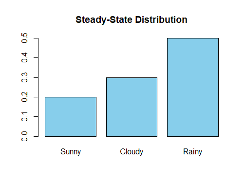
Markov Models. Using R

Simulation Plots: Plots generated from model simulations, demonstrating the evolution of states over time under different scenarios.

R

# Example using ggplot2 with simulated data
install.packages("ggplot2")
library(ggplot2)

set.seed(123)
simulated_data <- data.frame(Time = 1:10, State = sample(c("Sunny", "Cloudy", "Rainy"),
                                                         10, replace = TRUE))

ggplot(data = simulated_data, aes(x = Time, y = State, color = State)) +
  geom_point() +
  geom_line() +
  labs(title = "State Evolution Over Time", x = "Time", y = "State") +
  theme_minimal()

Output:

Markov Models. Using R

These visualization techniques help researchers, analysts, and users comprehend the intricate dynamics of Markov models and make informed interpretations.

Challenges of Markov Models

• Dependency Assumption:- Events depend only on the current state, potentially overlooking the influence of past events.
• Sensitivity to Starting Conditions:- Small changes in initial conditions or transition probabilities can significantly impact predictions.
• Memoryless Behavior:- Relies on the current state, disregarding the historical sequence of events.
• Limited Representation:- Markov Models may struggle to capture intricate relationships within a system.
• Stationarity Assumption:- Assumes a stable environment, which may not hold in dynamic systems.
• Dimensionality Issues:- Handling a large number of states can pose computational challenges.

Markov Models Vs Other modeling approaches

Feature	Markov Models	Other Models (e.g., Regression, Neural Networks)
Modeling Assumption	Future state depends only on current state	Dependent on the chosen model structure and parameters
Temporal Dynamics	Captures sequential dependencies	May or may not explicitly capture temporal dependencies
Memoryless Property	Memoryless (next state independent of past states given current state)	May or may not exhibit memoryless property
State Transition Probabilities	Transition probabilities explicitly defined	No explicit transition probabilities, learned from data
Training Data	Requires historical state transitions	Requires input-output pairs, may include time series data
Applications	Natural language processing, Finance, Biology	Predictive modeling, classification, regression
Interpretability	Transparent, easy to interpret	Interpretability varies based on model complexity
Handling Missing Data	Can handle missing transitions in some cases	Handling depends on the specific model and imputation methods
Complexity	Simplicity in structure, suitable for certain scenarios	Can handle complex relationships, may require larger datasets
Data Requirements	Sensitive to the quality of historical data	Relatively flexible, can handle missing or noisy data
Computation	Generally computationally efficient	Computationally expensive for complex models or large datasets

Future Developments in Markov Models

1. Enhanced Model Flexibility:- Future models may explore adaptive structures, allowing for more dynamic representation of evolving systems.
2. Improve Machine Learning Techniques:- Integration with machine learning approaches could enhance Markov models, improving predictive accuracy and handling complex data patterns.
3. Handling Non-Stationary Environments:- Future developments may focus on models capable of adapting to changing environments, challenging the traditional stationarity assumption.
4. Improved Transition Probability Estimation:- Advancements in estimation techniques may address challenges in accurately determining transition probabilities, especially in intricate systems.
5. Efficient Handling of Large State Spaces:- Developments in computational methods may address challenges associated with dimensionality, enabling the application of Markov models in larger state spaces.
6. Hybrid Models for Varied Applications:- Future developments may explore hybrid models, combining Markov models with other probabilistic methods for improved applicability across diverse domains.
7. Continuous-Time Model Refinement:- Advancements in continuous-time modeling may refine techniques for seamlessly integrating Markov models into time-sensitive processes.

Conclusion

Markov Models are key in understanding sequences, while R’s markovchain package boosts this analysis. R makes Markov Models accessible, shedding light on trends in finance, biology, and marketing, aiding better choices.

Across academia, finance, and healthcare, R’s user-friendliness merges seamlessly with Markov Models’ flexibility, making predictive analytics accessible. This blend sparks innovation and smart decision-making in various industries.