Machine Learning is an important part of Artificial Intelligence for data analysis. It is widely used in many sectors such as healthcare, E-commerce, Finance, Recommendations, etc. It plays an important role in understanding the trends and patterns in our data to predict useful information that can be used for better decision-making.
There are three types of machine learning:
- Supervised Machine Learning
- Unsupervised Machine Learning
- Reinforcement Machine Learning
In supervised Machine Learning the algorithm learns from the labelled dataset and the goal is to map the input and output from the data to predict future values. In R programming Language It is widely used in various applications such as Regression and Classification to solve real-world issues.
- Regression: This type of model focuses on building relationships between the variables. For example, the prediction of house price based on other variables such as size or location comes under regression.
- Classification: This model involves categorizing data into predefined classes. This type of model is used in email spam detection. Data miners and researchers use ML for predictive analysis and this analysis is made easier by the R programming Language. R is a language that provides a wide range of packages to help in data analysis and predictions. One such package is “caret”. In this article, we will try to understand how to use caret in Supervised Machine Learning by training and tuning ML models with the help of multiple examples.
Understanding Training and Tuning
Training and Tuning is an important part of building a machine learning model which is aimed at achieving optimal performance of the model. This is a process in which the model is trained to perform and then fine tuning is done to check the parameters to improve its predictability.
- Training of the model: To train an ML model we must select the appropriate data and deal with it before processing it. After handling the missing values, scaling, and splitting data into training and tuning sets we must choose the perfect algorithm we start the training of the model. The model is then trained using the training data, and the algorithm learns the underlying patterns and relationships within the data.
- Tuning of the model: Tuning of the model involves dealing with hyperparameters. Hyperparameters are the configuration settings that are not learned directly from the data during training and they impact the performance of the model. Tuning these models is necessary to improve the performance of the model. Techniques such as grid search, random search, and Bayesian optimization are commonly used for this purpose.
Overview of caret Package
Caret is a powerful package in R which stands for Classification And Regression Training. It is a versatile tool since it provides a wide range of predictive modeling in both classification and regression. This package helps the analyst to experiment without issues of learning multiple algorithms.
To install this package we can use the following command in our R environment.
#installing the package
install.packages("caret")
- Simplified Learning: caret helps in dealing with different machine learning models without knowing each of them in detail.
- Preprocessing Capabilities: We face a lot of errors when we have missing values in our dataset generally when we deal with large data, caret helps in making the data ready by fixing such errors.
- Model Training and Tuning: It helps in creating models that we will learn further in this article.
- Model Evaluation: It also evaluates the model and tells if it needs any correction giving stats of our model.
Training and Tuning Models with Caret
- Training: Training means dealing with the dataset and training it to make useful predictions or future data.
- Tuning: Tuning means selecting the best parameters for the algorithm to maximize its performance.
We will follow certain steps in this article to train and tune our model.
- Data Preparation
- Model Training
- Model Tuning
- Making Prediction
- Visualization
We will follow these steps and try to understand caret with the help of multiple examples.
Retail – Demand Forecasting
In this example. we will create our fictional dataset on Retail – Demand Forecasting using a set.seed() function that generates random numbers for our dataset but before that, we will load the necessary packages and also check for missing values since it can alter our prediction and training.
Load the package
R
library(caret)
library(ggplot2
|
Step 1: Load and preprocess the dataset
Generating a fictional dataset
R
set.seed(123)
retail_data <- data.frame(
sales = round(rnorm(100, mean = 100, sd = 20)),
price = round(runif(100, min = 50, max = 200)),
advertising = round(runif(100, min = 500, max = 2000))
)
retail_data[sample(1:100, 10), "sales"] <- NA
head(retail_data)
|
Output:
  sales price advertising
1    89    86        1677
2    95   194         514
3   131   140        1669
4   101   127        1594
5   103   110        1445
6   134   182        1221
Check for missing values
R
sum(is.na(retail_data$sales))
|
Output:
[1] 10
Impute missing values
R
retail_data$sales[is.na(retail_data$sales)] <- mean(retail_data$sales, na.rm = TRUE)
|
Step 2: Model Training
Here we defined the control parameters cv with five folds. cv here means cross-validation method.
Other sampling method is bootstrap. Both of these are resampling techniques used in statistical analysis of our models.
Cross- validation : This involves dividing the data into multiple subsets or folds. This method is used in ML modeling when the dataset is limited.
Bootstrap: This technique involves generating multiple samples with replacement from the original dataset. It is created randomly from the original dataset with replacement.
lm() function is used to train the linear regression model.
Model Training with Cross-Validation using caret
R
control_cv <- trainControl(method = "cv", number = 5)
model_cv <- train(sales ~ price + advertising, data = retail_data, method = "lm",
trControl = control_cv)
cat("Results from Model Training with Cross-Validation:")
print(model_cv)
|
Output:
Results from Model Training with Cross-Validation:
Linear Regression

100 samples
  2 predictor

No pre-processing
Resampling: Cross-Validated (5 fold)
Summary of sample sizes: 79, 81, 80, 80, 80
Resampling results:

  RMSE      Rsquared    MAE
  17.36428  0.03777004  13.98392

Tuning parameter 'intercept' was held constant at a value of TRUE
- method= lm is used indicating the linear regression model.
- The dataset contains 100 sample values and 2 predicter variables namely price and advertising.
- This model is evaluated using 5 folds of cross validation and 50 reps for bootstrap.
- The sample sizes of each of the five folds are then given as summary which are, 79, 81, 80, 80, 80 respectively for cv and 100 each for bootstrap technique.
- RMSE: Root mean squared error indicates the average difference between the actual and predicted values, which is 17.36 here for cv resampling showing the deviation of prediction from actual sales.
- Rsquared (R²): It indicates the proportion of variance in the dependent variable from the independent variable. The output value is small therefore the model explains only a small portion of variance.
- MAE (Mean Absolute Error): It indicates the average absolute difference between the actual and predicted values.
Summary of the model
R
cat("\n Summary of the model")
summary(model_cv)
|
Output:
 Summary of the model

Call:
lm(formula = .outcome ~ ., data = dat)

Residuals:
    Min      1Q  Median      3Q     Max
-44.957 -12.060  -0.138  10.930  41.893

Coefficients:
             Estimate Std. Error t value Pr(>|t|)
(Intercept) 93.536536   7.101323  13.172   <2e-16 ***
price        0.030053   0.040647   0.739    0.461
advertising  0.003834   0.004067   0.943    0.348
---
Signif. codes:  0 ‘***’ 0.001 ‘**’ 0.01 ‘*’ 0.05 ‘.’ 0.1 ‘ ’ 1

Residual standard error: 17.8 on 97 degrees of freedom
Multiple R-squared:  0.01549,    Adjusted R-squared:  -0.004813
F-statistic: 0.7629 on 2 and 97 DF,  p-value: 0.4691
Model Training using Bootstrap Resampling in caret
R
control_boot <- trainControl(method = "boot", number = 50)
model_boot <- train(sales ~ price + advertising, data = retail_data, method = "lm",
trControl = control_boot)
cat("Results from Model Training with Bootstrap Resampling:")
print(model_boot)
|
Output:
Results from Model Training with Bootstrap Resampling:
Linear Regression

100 samples
  2 predictor

No pre-processing
Resampling: Bootstrapped (50 reps)
Summary of sample sizes: 100, 100, 100, 100, 100, 100, ...
Resampling results:

  RMSE      Rsquared    MAE
  18.74339  0.02072637  14.76535

Tuning parameter 'intercept' was held constant at a value of TRUE
Print the summary of the model
R
cat("\n Summary of the model")
summary(model_cv)
|
Output:
 Summary of the model

Call:
lm(formula = .outcome ~ ., data = dat)

Residuals:
    Min      1Q  Median      3Q     Max
-44.957 -12.060  -0.138  10.930  41.893

Coefficients:
             Estimate Std. Error t value Pr(>|t|)
(Intercept) 93.536536   7.101323  13.172   <2e-16 ***
price        0.030053   0.040647   0.739    0.461
advertising  0.003834   0.004067   0.943    0.348
---
Signif. codes:  0 ‘***’ 0.001 ‘**’ 0.01 ‘*’ 0.05 ‘.’ 0.1 ‘ ’ 1

Residual standard error: 17.8 on 97 degrees of freedom
Multiple R-squared:  0.01549,    Adjusted R-squared:  -0.004813
F-statistic: 0.7629 on 2 and 97 DF,  p-value: 0.4691
Step 3: Model Tuning
This part tunes the model to improve its performance. Here we are using additional parameters to tune the model by grid search and random search method. The caret package in R supports these two search methods.
Random Search Method:
Random Search Method is not s systematic approach, on the other hand, this randomly samples points from the specified search space of hyperparameters. it does not extensively apply all the combination which makes it suitable for the large datasets. It is used when the relationship between hyperparameters and model performance is complex and poorly understood.
R
set.seed(123)
tuned_model_random <- train(sales ~ price + advertising, data = retail_data, method = "lm",
trControl = control_boot, tuneGrid = data.frame(intercept = TRUE),
tuneLength = 5)
print("Results from Random Search Tuning:")
print(tuned_model_random)
|
Output:
[1] "Results from Random Search Tuning:"
Linear Regression

100 samples
  2 predictor

No pre-processing
Resampling: Bootstrapped (50 reps)
Summary of sample sizes: 100, 100, 100, 100, 100, 100, ...
Resampling results:

  RMSE      Rsquared    MAE
  18.28558  0.01631783  14.31087

Tuning parameter 'intercept' was held constant at a value of TRUE
Grid Search Method:
Grid Search Method is a systematic approach of defining grid hyperparameters for the values that are supposed to be evaluated. It is beneficial when the relationship between hyperparameters and model performance is already known. It is not beneficial when we have a large dataset because typically the grid parameters are predefined and each combination is tested. This can be computationally costly therefore it is not suitable for large datasets.
R
set.seed(123)
grid <- expand.grid(.intercept = c(TRUE, FALSE))
set.seed(123)
tuned_model_grid <- train(sales ~ price + advertising, data = retail_data, method = "lm",
trControl = control_boot, tuneGrid = grid)
print("Results from Grid Search Tuning:")
print(tuned_model_grid)
|
Output:
[1] "Results from Grid Search Tuning:"
Linear Regression

100 samples
  2 predictor

No pre-processing
Resampling: Bootstrapped (50 reps)
Summary of sample sizes: 100, 100, 100, 100, 100, 100, ...
Resampling results across tuning parameters:

  intercept  RMSE      Rsquared    MAE
  FALSE      29.86268  0.02661813  24.62961
   TRUE      18.28558  0.01631783  14.31087

RMSE was used to select the optimal model using the smallest value.
The final value used for the model was intercept = TRUE.
By reading and understanding the statistics of both the tuning method we find that the model’s predicting ability is limited because of low rsquared value and relatively high RMSE AND MAE value.
We can also change the resampling technique from cross validation to bootstrap for our model tuning.
Bootstrap Resampling
For bootstrap resampling technique we can follow the code:
Tuning the model with Random Search and Bootstrap Resampling
R
control_random <- trainControl(method = "boot", number = 50)
grid_random <- data.frame(alpha = runif(10, 0, 1), lambda = runif(10, 0.01, 1))
tuned_model_random <- train(sales ~ price + advertising, data = retail_data,
method = "glmnet", trControl = control_random, tuneGrid = grid_random)
print("Results from Random Search Tuning with Bootstrap Resampling:")
print(tuned_model_random)
|
Output:
[1] "Results from Random Search Tuning with Bootstrap Resampling:"
glmnet

100 samples
  2 predictor

No pre-processing
Resampling: Bootstrapped (50 reps)
Summary of sample sizes: 100, 100, 100, 100, 100, 100, ...
Resampling results across tuning parameters:

  alpha       lambda      RMSE      Rsquared    MAE
  0.03363409  0.21612625  18.21563  0.02693100  14.39546
  0.20290364  0.16135748  18.21249  0.02686727  14.39186
  0.26269758  0.28128161  18.19998  0.02681105  14.37700
  0.37292502  0.69286338  18.15357  0.02643586  14.31783
  0.38777702  0.15993315  18.20670  0.02682547  14.38503
  0.50749510  0.06191812  18.21649  0.02686557  14.39660
  0.62412407  0.44931432  18.15749  0.02649959  14.32198
  0.67755950  0.93917908  18.09118  0.02510399  14.22676
  0.75109712  0.18617982  18.19080  0.02667146  14.36569
  0.94719661  0.80162434  18.07792  0.02466289  14.20708

RMSE was used to select the optimal model using the smallest value.
The final values used for the model were alpha = 0.9471966 and lambda = 0.8016243.
Tuning the model with Grid Search with Bootstrap Resampling
R
library(glmnet)
control_grid <- trainControl(method = "boot", number = 50)
grid <- expand.grid(alpha = seq(0, 1, by = 0.1), lambda = seq(0.01, 1, by = 0.1))
tuned_model_grid <- train(sales ~ price + advertising, data = retail_data,
method = "glmnet", trControl = control_grid, tuneGrid = grid)
print("Results from Grid Search Tuning with Bootstrap Resampling:")
print(tuned_model_grid)
|
Output:
[1] "Results from Grid Search Tuning with Bootstrap Resampling:"
glmnet

100 samples
  2 predictor

No pre-processing
Resampling: Bootstrapped (50 reps)
Summary of sample sizes: 100, 100, 100, 100, 100, 100, ...
Resampling results across tuning parameters:

  alpha  lambda  RMSE      Rsquared    MAE
  0.0    0.01    18.25627  0.01943666  14.34203
  0.0    0.11    18.25627  0.01943679  14.34203
  0.0    0.21    18.25605  0.01944021  14.34182
  0.0    0.31    18.25508  0.01944550  14.34072
  0.0    0.41    18.25335  0.01945157  14.33877
  0.0    0.51    18.25102  0.01945723  14.33624
  0.0    0.61    18.24814  0.01946256  14.33309
  0.0    0.71    18.24530  0.01946784  14.32999
  0.0    0.81    18.24251  0.01947306  14.32693
  0.0    0.91    18.23976  0.01947823  14.32390
  0.1    0.01    18.26278  0.01942244  14.34904
  0.1    0.11    18.26085  0.01942853  14.34710
  0.1    0.21    18.25582  0.01942962  14.34171
  0.1    0.31    18.25089  0.01943233  14.33642
  0.1    0.41    18.24607  0.01943270  14.33129
  0.1    0.51    18.24140  0.01942442  14.32629
  0.1    0.61    18.23682  0.01941665  14.32134
  0.1    0.71    18.23232  0.01940918  14.31647
  0.1    0.81    18.22789  0.01940588  14.31169
  0.1    0.91    18.22351  0.01942140  14.30699
  0.2    0.01    18.26288  0.01941806  14.34913
  0.2    0.11    18.25866  0.01942336  14.34482
  0.2    0.21    18.25173  0.01942073  14.33745
  0.2    0.31    18.24508  0.01939929  14.33045
  0.2    0.41    18.23853  0.01938870  14.32352
  0.2    0.51    18.23205  0.01941876  14.31671
  0.2    0.61    18.22572  0.01945665  14.31003
  0.2    0.71    18.21957  0.01950266  14.30356
  0.2    0.81    18.21357  0.01955869  14.29718
  0.2    0.91    18.20776  0.01962381  14.29080
  0.3    0.01    18.26293  0.01941598  14.34918
  0.3    0.11    18.25648  0.01941998  14.34254
  0.3    0.21    18.24780  0.01939250  14.33344
  0.3    0.31    18.23926  0.01939722  14.32452
  0.3    0.41    18.23089  0.01944902  14.31582
  0.3    0.51    18.22279  0.01951975  14.30733
  0.3    0.61    18.21494  0.01961320  14.29904
  0.3    0.71    18.20741  0.01971809  14.29067
  0.3    0.81    18.20000  0.01970757  14.28232
  0.3    0.91    18.19272  0.01964209  14.27425
  0.4    0.01    18.26297  0.01941642  14.34923
  0.4    0.11    18.25435  0.01941250  14.34031
  0.4    0.21    18.24383  0.01938184  14.32941
  0.4    0.31    18.23345  0.01944605  14.31869
  0.4    0.41    18.22345  0.01954464  14.30827
  0.4    0.51    18.21387  0.01968357  14.29800
  0.4    0.61    18.20457  0.01969879  14.28766
  0.4    0.71    18.19544  0.01961000  14.27756
  0.4    0.81    18.18655  0.01951222  14.26774
  0.4    0.91    18.17794  0.01939244  14.25815
  0.5    0.01    18.26295  0.01941640  14.34922
  0.5    0.11    18.25227  0.01939728  14.33819
  0.5    0.21    18.23982  0.01940925  14.32538
  0.5    0.31    18.22775  0.01951492  14.31291
  0.5    0.41    18.21623  0.01968260  14.30070
  0.5    0.51    18.20511  0.01966954  14.28839
  0.5    0.61    18.19421  0.01955526  14.27642
  0.5    0.71    18.18368  0.01941538  14.26482
  0.5    0.81    18.17351  0.01921789  14.25347
  0.5    0.91    18.16399  0.01888988  14.24217
  0.6    0.01    18.26300  0.01941667  14.34928
  0.6    0.11    18.25019  0.01938302  14.33607
  0.6    0.21    18.23586  0.01944492  14.32141
  0.6    0.31    18.22215  0.01960828  14.30717
  0.6    0.41    18.20912  0.01968752  14.29294
  0.6    0.51    18.19637  0.01954914  14.27893
  0.6    0.61    18.18408  0.01937374  14.26546
  0.6    0.71    18.17232  0.01909617  14.25227
  0.6    0.81    18.16150  0.01880447  14.23922
  0.6    0.91    18.15169  0.01874581  14.22652
  0.7    0.01    18.26297  0.01941694  14.34926
  0.7    0.11    18.24809  0.01937288  14.33396
  0.7    0.21    18.23196  0.01948982  14.31744
  0.7    0.31    18.21671  0.01970455  14.30135
  0.7    0.41    18.20200  0.01959250  14.28520
  0.7    0.51    18.18780  0.01940098  14.26969
  0.7    0.61    18.17424  0.01908563  14.25462
  0.7    0.71    18.16188  0.01876927  14.23975
  0.7    0.81    18.15092  0.01873810  14.22528
  0.7    0.91    18.14097  0.01833118  14.21129
  0.8    0.01    18.26296  0.01941820  14.34925
  0.8    0.11    18.24597  0.01938180  14.33183
  0.8    0.21    18.22809  0.01954601  14.31352
  0.8    0.31    18.21128  0.01967945  14.29544
  0.8    0.41    18.19497  0.01948635  14.27759
  0.8    0.51    18.17940  0.01919003  14.26057
  0.8    0.61    18.16512  0.01879351  14.24380
  0.8    0.71    18.15263  0.01873553  14.22748
  0.8    0.81    18.14148  0.01716739  14.21169
  0.8    0.91    18.13137  0.01592892  14.19646
  0.9    0.01    18.26296  0.01941897  14.34927
  0.9    0.11    18.24384  0.01939586  14.32970
  0.9    0.21    18.22428  0.01961356  14.30958
  0.9    0.31    18.20583  0.01960790  14.28954
  0.9    0.41    18.18806  0.01935490  14.27019
  0.9    0.51    18.17136  0.01884871  14.25142
  0.9    0.61    18.15687  0.01873875  14.23317
  0.9    0.71    18.14418  0.01832623  14.21537
  0.9    0.81    18.13287  0.01592702  14.19840
  0.9    0.91    18.12221  0.01622801  14.18179
  1.0    0.01    18.26295  0.01941927  14.34928
  1.0    0.11    18.24173  0.01941223  14.32759
  1.0    0.21    18.22055  0.01969121  14.30562
  1.0    0.31    18.20044  0.01953153  14.28367
  1.0    0.41    18.18126  0.01917529  14.26281
  1.0    0.51    18.16395  0.01875248  14.24243
  1.0    0.61    18.14933  0.01832831  14.22257
  1.0    0.71    18.13654  0.01591612  14.20370
  1.0    0.81    18.12461  0.01621952  14.18524
  1.0    0.91    18.11374  0.01619176  14.16821

RMSE was used to select the optimal model using the smallest value.
The final values used for the model were alpha = 1 and lambda = 0.91.
We can also plot these values for better visualization for coefficient. This plot displays the estimated coefficients of the predictor variables in the linear regression model. It helps to understand the impact of each variable on the target variable (sales).
It helps identify patterns in the residuals and assess the linearity assumption. The horizontal line at 0 indicates the absence of systematic patterns.
Coefficient plot for Cross-Validation model
R
coeff_plot <- plot(model_cv$finalModel, col = "darkgreen", main = "Coefficient Plot")
|
Output:

Residuals vs Fitted
Another code is for Q-Q residual graph that we will plot to understand the parameters. A quantile-quantile plot compares the distribution of standardized residuals to a theoretical normal distribution. If the points closely follow the line which is diagonal then it means that the residuals are approximately normally distributed.
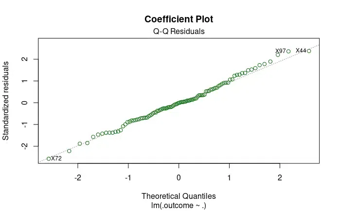
Q-Q Residuals
The third plot for this code is for scale location. This is also known as Spread-Location plot, it examines the spread of standardized residuals against the fitted values.
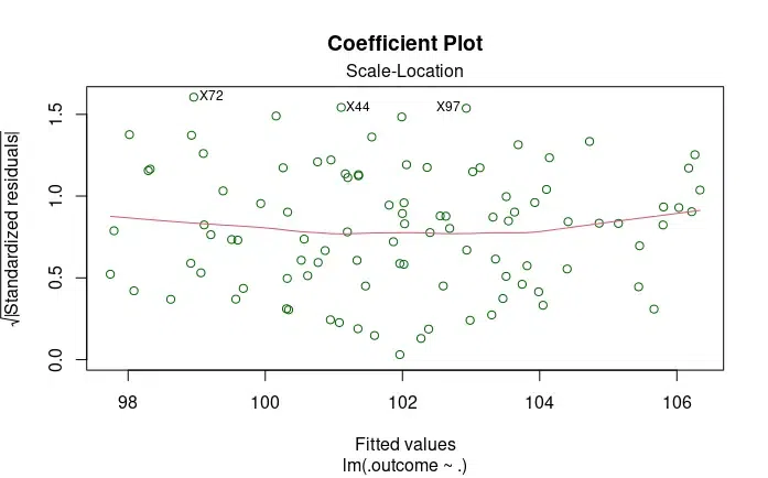
Scale-Location
Standardized Residuals: These are the residuals (differences between observed and predicted values) standardized by their estimated standard deviation.
Leverage: A measure of how much an observation influences the fit of the model. High leverage points can have a substantial impact on the regression coefficients.
Cook’s Distance: It quantifies how much the predicted values (fitted values) would change if a particular observation is excluded from the dataset.
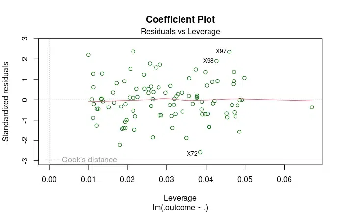
Residuals vs Leverage
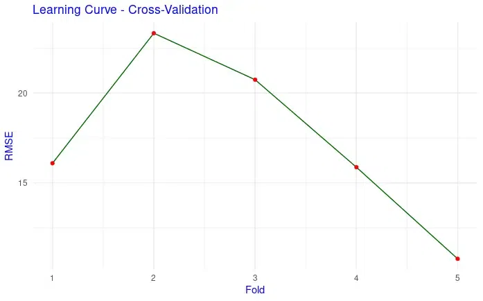
Learning Curve
Another Graph that we can plot is the learning curve. This learning curve shows the training error (RMSE) across different folds during cross-validation. It helps to assess how well the model is learning from the training data and if there is overfitting or underfitting.
R
learning_curve <- data.frame(TrainError = model_cv$resample$RMSE,
TestError = model_cv$resample$Rsquared)
ggplot(learning_curve, aes(x = seq_along(TrainError), y = TrainError, group = 1)) +
geom_line(color = "darkgreen") +
geom_point(color = "red") +
labs(x = "Fold", y = "RMSE", title = "Learning Curve - Cross-Validation") +
theme_minimal() +
theme(text = element_text(color = "blue"))
|
Output:
RMSE per Fold
Step 4: Making Predictions
We will make predictions for only last 10 rows to analyze the data by using predict() function.
Predictions with Random Model
R
predictions <- predict(tuned_model_random, retail_data[1:10, ])
print(predictions)
|
Output:
        1         2         3         4         5         6         7         8
102.43532 101.36146 103.15826 102.81523 102.25478 102.75005 100.62648  99.97203
        9        10
101.20417 101.33379
Making predictions with grid model
R
predictions <- predict(tuned_model_grid, retail_data[1:10, ])
print(predictions)
|
Output:
       1        2        3        4        5        6        7        8        9
102.4138 101.3644 102.9661 102.6887 102.2303 102.5660 100.8444 100.2995 101.3735
      10
101.4844
These are the output of predicted sales of the first 10 rows. For example, the first value, 102.55030, represents the predicted sales for the first data point similarly all the sales is for the corresponding data point.
Step 5: Visualization
R
ggplot(retail_data, aes(x = price, y = sales)) +
geom_point(color = "darkgreen") +
geom_smooth(method = "lm", se = FALSE, color = "green") +
labs(x = "Price", y = "Sales", title = "Retail Demand best fit line") +
theme_minimal() +
theme(text = element_text(color = "green"))
|
Output:
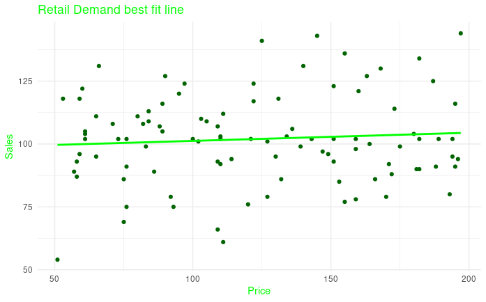
Retail Demand best fit line
The dots in dark green represent the data points from our dataset and the line shows the regression fit of our model. This plot shows the relationship between sales and price.
We can also plot the actual and predicted sales on the graph:
R
predicted_cv <- predict(model_cv)
actual_cv <- retail_data$sales
plot(x = actual_cv, y = predicted_cv, col = "darkgreen", pch = 16,
main = "Predicted vs Actual Sales", xlab = "Actual Sales", ylab = "Predicted Sales")
abline(a = 0, b = 1, col = "red", lty = 2)
|
Output:
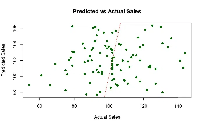
In this example, we generated a retail dataset with 100 observations. Using caret package in R language we predicted the values and performed training and tuning model and finally plotted the graph for the same. The price and sales estimation helps retailers in better decision making about their stock and sales.
Conclusion
In this article, We used “caret” library in R language to train and tune our model and understood its features. We also plotted the graph of the examples to understand them in visual manner. We understood the concept with the help of example and plotted the results for the same.
Share your thoughts in the comments
Please Login to comment...