Difference between Distance vector routing and Link State routing

Prerequisite – Classification of Routing Algorithms

Distance Vector Routing –

• It is a dynamic routing algorithm in which each router computes a distance between itself and each possible destination i.e. its immediate neighbors.
• The router shares its knowledge about the whole network to its neighbors and accordingly updates the table based on its neighbors.
• The sharing of information with the neighbors takes place at regular intervals.
• It makes use of Bellman-Ford Algorithm for making routing tables.
• Problems – Count to infinity problem which can be solved by splitting horizon. 
  – Good news spread fast and bad news spread slowly. 
  – Persistent looping problem i.e. loop will be there forever.

Link State Routing –

• It is a dynamic routing algorithm in which each router shares knowledge of its neighbors with every other router in the network.
• A router sends its information about its neighbors only to all the routers through flooding.
• Information sharing takes place only whenever there is a change.
• It makes use of Dijkstra’s Algorithm for making routing tables.
• Problems – Heavy traffic due to flooding of packets. 
  – Flooding can result in infinite looping which can be solved by using the Time to live (TTL) field. 

Comparison between Distance Vector Routing and Link State Routing: 

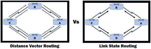
Figure:- Distance Vector Routing Vs Link State Routing

S.No.	Distance Vector Routing	Link State Routing
1.	Bandwidth required is less due to local sharing, small packets and no flooding.	Bandwidth required is more due to flooding and sending of large link state packets.
2.	Based on local knowledge, since it updates table based on information from neighbours.	Based on global knowledge, it have knowledge about entire network.
3.	Make use of Bellman Ford Algorithm.	Make use of Dijakstra’s algorithm.
4.	Traffic is less.	Traffic is more.
5.	Converges slowly i.e, good news spread fast and bad news spread slowly.	Converges faster.
6.	Count of infinity problem.	No count of infinity problem.
7.	Persistent looping problem i.e, loop will be there forever.	No persistent loops, only transient loops.
8.	Practical implementation is RIP and IGRP.	Practical implementation is OSPF and ISIS.

My Personal Notes arrow_drop_up

Save