Non Parametric Density Estimation Methods in Machine Learning

Non-parametric methods: Similar inputs have similar outputs. These are also called instance-based or memory-based learning algorithms. There are 4 Non – parametric density estimation methods:

1. Histogram Estimator
2. Naive Estimator
3. Kernel Density Estimator (KDE)
4. KNN estimator (K – Nearest Neighbor Estimator)

Histogram Estimator

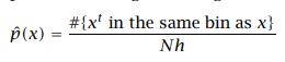
It is the oldest and the most popular method used to estimate the density, where the input space is divided into equal-sized intervals called bins. Given the training set X = {x^t}^N _t=1 an origin x₀ and the bin width h, the histogram density estimator function is:

Histogram estimator

The density of a sample is dependent on the number of training samples present in that bin. In constructing the histogram of densities we choose the origin and the bin width, the position of origin affects the estimation near the boundaries.

Python3

import numpy as np

def hist_pdf(x, data, n_bins=2,
             minv=None, maxv=None):
    if minv is None:
        minv = np.min(data)
    if maxv is None:
        maxv = np.max(data)
    d = (maxv-minv) / n_bins
    bins = np.arange(minv, maxv, d)
    bin_id = int((x-minv)/d)
    bin_minv = minv+d*bin_id
    bin_maxv = minv+d*(bin_id+1)
    n_data = len(data)
    y = len(data[np.where((data > bin_minv)\
                          & (data < bin_maxv))])
    pdf = (1.0/d) * (y / n_data)
    return pdf

Now, let’s plot a histogram for the histogram Estimator.

Python3

from sklearn.datasets import load_boston
import matplotlib.pyplot as plt
ds = load_boston()
data = ds['target']
# Demo histogram
xvals = np.arange(min(data), max(data), 1)
n_bins = 15
pdf = [hist_pdf(x, data, n_bins=n_bins) for x in xvals]
plt.xlabel('Data')
plt.ylabel('Density')
plt.title('Histogram Density Estimation')
plt.plot(xvals, pdf)
plt.show()

Output:

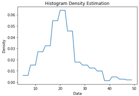
Histogram Density Estimation Plot

Naive Estimator

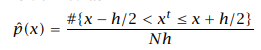
Unlike the Histogram estimator, the Naive estimator does not use the concept of origin. There is no assumption of choosing the origin. The density of the sample depends on the neighboring training samples. Given the training set X = {x^t}^N_t=1 and the bin width h, the Naive density estimator function is:

Naive estimator

The values in the range of h/2 to the left and right of the sample involve the density contribution.

Python3

import numpy as np

def naive_pdf(x, data, n_bins=2,
              minv=None, maxv=None):
    if minv is None:
        minv = np.min(data)
    if maxv is None:
        maxv = np.max(data)
    d = (maxv-minv) / n_bins
    bins = np.arange(minv, maxv, d)
    bin_id = int((x-minv)/d)
    bin_minv = minv+d*bin_id
    bin_maxv = minv+d*(bin_id+1)
    n_data = len(data)
    y = len(data[np.where((data > bin_minv//2)\
                          & (data < bin_maxv//2))])
    pdf = (1.0/d) * (y / n_data)
    return pdf

Now we will use the above function to plot a Naive Estimator graph.

Python3

from sklearn.datasets import load_boston
import matplotlib.pyplot as plt
ds = load_boston()
data = ds['target']
# Demo histogram
xvals = np.arange(min(data), max(data), 1)
n_bins = 15
pdf = [naive_pdf(x, data, n_bins=n_bins)\
       for x in xvals]
plt.xlabel('Data')
plt.ylabel('Density')
plt.title('Naive Density Estimation')
plt.plot(xvals, pdf)
plt.show()

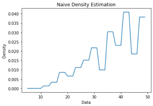
Naive Density Estimation plot

Kernel Density Estimator (KDE)

Kernel estimator is used to smoothen the probability distribution function (pdf) and cumulative distribution function (CDF) graphics. The kernel is nothing but a weight. Gaussian Kernel is the most popular kernel: 

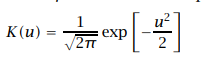
Gaussian kernel

The kernel estimator is also called Parzen Window:

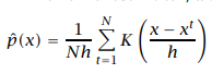
Kernel density estimator

As you can observe, as |x – x^t| increases that means, the training sample is far away from the given sample, and the kernel value decreases. Hence we can say that the contribution of a farther sample is less when compared to the nearest training samples. There are many more kernels: Gaussian, Rectangular, Triangular, Biweight, Uniform, Cosine, etc.

Python3

import numpy as np
from scipy.stats import norm
from sklearn.neighbors import KernelDensity
# Kernel Density Estimator using gaussian kernel
X = np.random.randn(100)
model = KernelDensity(kernel='gaussian',
                      bandwidth=0.2)
model.fit(X[:, None])
new_data = np.linspace(-5, 5, 1000)
density = np.exp(model.score_samples(new_data[:, None]))
# print(new_data)
# Plot the densities
plt.plot(new_data, density, '-',
         color='red')
plt.xlabel('Data')
plt.ylabel('Density')
plt.title('Kernel Density Estimator using Gaussian kernel')
plt.show()

Output:

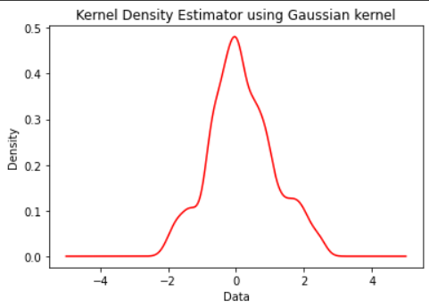
KDE plot using Gaussian Kernel 

K – Nearest Neighbor Estimator (KNN Estimator)

Unlike the previous methods of fixing the bin width h, in this estimation, we fix the value of nearest neighbors k. The density of a sample depends on the value of k and the distance of the kth nearest neighbor from the sample. This is close enough to the Kernel estimation method. The K-NN density estimation is, where d_k(x) is the Euclidean distance from the sample to its k^th nearest neighbor.

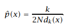
KNN Estimator

Let us have an example data sample and estimate the density at a point using nonparametric density estimation functions.

Note: Points marked with ‘x’ are the given data samples. Unlike the above estimation methods, we do not fix the bind size/width, instead, this density estimation method is based on the k value.  We observe a high-density value when k is less and the density is less when the value of k increases.

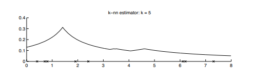
KNN Estimator

Python3

# KNN Density esitmator
gaussian = norm(loc=0.5, scale=0.2)
X = gaussian.rvs(500)
grid = np.linspace(-0.1, 1.1, 1000)
k_set = [5, 10, 20]
fig, axes = plt.subplots(3, 1, figsize=(10, 10))
for i, ax in enumerate(axes.flat):
    K = k_set[i]
    p = np.zeros_like(grid)
    n = X.shape[0]
    for i, x in enumerate(grid):
        dists = np.abs(X-x)
        neighbours = dists.argsort()
        neighbour_K = neighbours[K]
        p[i] = (K/n) * 1/(2 * dists[neighbour_K])
    ax.plot(grid, p, color='orange')
    ax.set_title(f'$k={K}$')
plt.show()

Output:

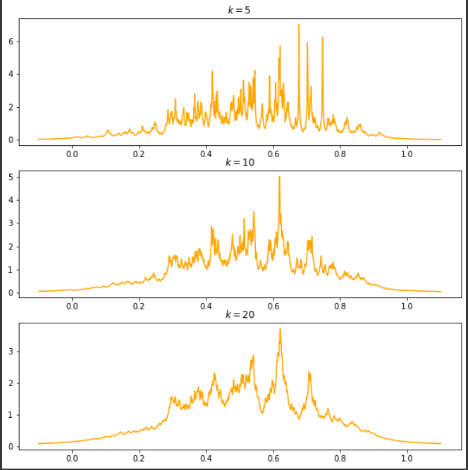
KNN Density Plots