Agglomerative Methods in Machine Learning

Before diving into the Agglomerative algorithms, we must understand the different concepts in clustering techniques. So, first, look at the concept of Clustering in Machine Learning:

Clustering is the broad set of techniques for finding subgroups or clusters on the basis of characterization of objects within dataset such that objects with groups are similar but different from the object of other groups. Primary guideline of clustering is that data inside a cluster should be very similar to each other but very different from those outside clusters. There are different types of clustering techniques like Partitioning Methods, Hierarchical Methods and Density Based Methods. 

Method	Characteristics
Partitioning Method	Uses mean/mediod to represent cluster centre Adopts distance-based approach to refine clusters Finds mutually exclusive clusters of spherical / nearly spherical shape Effective for datasets of small – medium age
Hierarchical Method	Creates tree-like structure through decomposition Uses distance between nearest / furthest points in neighbouring clusters for refinement Error can’t be corrected at subsequent levels
Density Based Method	Useful for identifying arbitrarily shaped clusters May filter out outliers

In Partitioning methods, there are 2 techniques namely, k-means and k-medoids technique ( partitioning around medoids algorithm ). But in order to learn about the Agglomerative Methods, we have to discuss the hierarchical methods.

• Hierarchical Methods: Data is grouped into a tree like structure. There are two main clustering algorithms in this method:
  • A. Divisive Clustering: It uses the top-down strategy, the starting point is the largest cluster with all objects in it and then split recursively to form smaller and smaller clusters. It terminates when the user-defined condition is achieved or final clusters contain only one object.
  • B. Agglomerative Clustering: It uses a bottom-up approach. It starts with each object forming its own cluster and then iteratively merges the clusters according to their similarity to form large clusters. It terminates either
    • When certain clustering condition imposed by user is achieved or
    • All clusters merge into a single cluster

A dendrogram, which is a tree like structure, is used to represent hierarchical clustering. Individual objects are represented by leaf nodes and the clusters are represented by root nodes. A representation of dendrogram is shown in this figure:

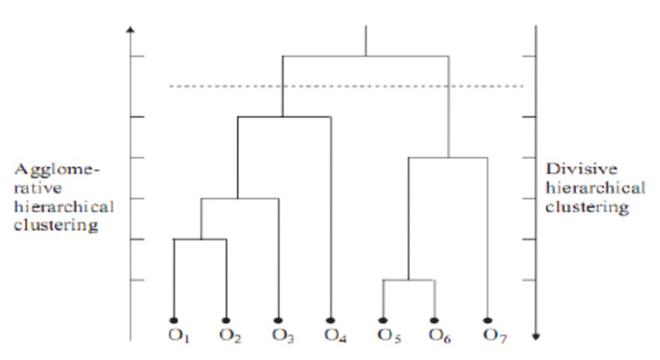
Dendrogram for Clustering

Now we will look into the variants of Agglomerative methods:

1. Agglomerative Algorithm: Single Link

Single-nearest distance or single linkage is the agglomerative method that uses the distance between the closest members of the two clusters. We will now solve a problem to understand it better:

Question. Find the clusters using a single link technique. Use Euclidean distance and draw the dendrogram.

Sample No.	X	Y
P1	0.40	0.53
P2	0.22	0.38
P3	0.35	0.32
P4	0.26	0.19
P5	0.08	0.41
P6	0.45	0.30

Solution:

Step 1: Compute the distance matrix by:  

So we have to find the Euclidean distance between each and every points, say we first find the euclidean distance between P1 and P2

 = 

So the DISTANCE MATRIX will look like this:

Similarly, find the Euclidean distance for every point. But there is one point to focus on that the diagonal of the above distance matrix is a special point for us. The distance above and below the diagonal will be same. For eg: d(P2, P5) is equivalent to d(P5, P2). So we will find the distance of the below section of the matrix. 

Therefore, the updated Distance Matrix will be :

Step 2: Merging the two closest members of the two clusters and finding the minimum element in distance matrix. Here the minimum value is 0.10 and hence we combine P3 and P6 (as 0.10 came in the P6 row and P3 column). Now, form clusters of elements corresponding to the minimum value and update the distance matrix. To update the distance matrix:

min ((P3,P6), P1) = min ((P3,P1), (P6,P1)) = min (0.22,0.24) = 0.22

min ((P3,P6), P2) = min ((P3,P2), (P6,P2)) = min (0.14,0.24) = 0.14

min ((P3,P6), P4) = min ((P3,P4), (P6,P4)) = min (0.13,0.22) = 0.13

min ((P3,P6), P5) = min ((P3,P5), (P6,P5)) = min (0.28,0.39) = 0.28

Now we will update the Distance Matrix:

Now we will repeat the same process. Merge two closest members of the two clusters and find the minimum element in distance matrix. The minimum value is 0.13 and hence we combine P3, P6 and P4. Now, form the clusters of elements corresponding to the minimum values and update the Distance matrix. In order to find, what we have to update in distance matrix,

min (((P3,P6) P4), P1) = min (((P3,P6), P1), (P4,P1)) = min (0.22,0.37) = 0.22

min (((P3,P6), P4), P2) = min (((P3,P6), P2), (P4,P2)) = min (0.14,0.19) = 0.14

min (((P3,P6), P4), P5) = min (((P3,P6), P5), (P4,P5)) = min (0.28,0.23) = 0.23

Now we will update the Distance Matrix:

Again repeating the same process: The minimum value is 0.14 and hence we combine P2 and P5. Now, form cluster of elements corresponding to minimum value and update the distance matrix. To update the distance matrix:

min ((P2,P5), P1) = min ((P2,P1), (P5,P1)) = min (0.23, 0.34) = 0.23

min ((P2,P5), (P3,P6,P4)) = min ((P3,P6,P4), (P3,P6,P4)) = min (0.14. 0.23) = 0.14

Update Distance Matrix will be:

Again repeating the same process: The minimum value is  0.14 and hence we combine P2,P5 and P3,P6,P4. Now, form cluster of elements corresponding to minimum value and update the distance matrix. To update the distance matrix:

min ((P2,P5,P3,P6,P4), P1) = min ((P2,P5), P1), ((P3,P6,P4), P1)) = min (0.23, 0.22) = 0.22

Updated Distance Matrix will be:

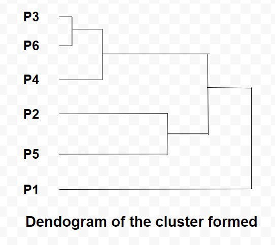
So now we have reached to the solution finally, the dendrogram for those question will be as follows:

2. Agglomerative Algorithm: Complete Link

In this algorithm, complete farthest distance or complete linkage is the agglomerative method that uses the distance between the members that are the farthest apart.

Question. For the given set of points, identify clusters using the complete link agglomerative clustering

Sample No	X	Y
P1	1	1
P2	1.5	1.5
P3	5	5
P4	3	4
P5	4	4
P6	3	3.5

Solution.

Step 1: Compute the distance matrix by:    So we have to find the euclidean distance between each and every point, say we first find the euclidean distance between P1 and P2.  (fORMULA FOR CALCULATING THE DISTANCE IS SAME AS ABOVE)

Say the Distance Matrix for  some points is :

Step 2: Merging the two closest members of the two clusters and finding the minimum element in distance matrix. So, the minimum value is 0.5 and hence we combine P4 and P6. To update the distance matrix,

max (d(P4,P6), P1) = max (d(P4,P1), d(P6,P1)) = max (3.6, 3.2) = 3.6

max (d(P4,P6), P2) = max (d(P4,P2), d(P6,P2)) = max (2.92, 2.5) = 2.92

max (d(P4,P6), P3) = max (d(P4,P3), d(P6,P3)) = max (2.24, 2.5) = 2.5

max (d(P4,P6), P5) = max (d(P4,P5), d(P6,P5)) = max (1.0, 1.12) = 1.12 

Updated distance matrix is:

Again, merging the two closest members of the two clusters and finding the minimum element in distance matrix. We get the minimum value as 0.71 and hence we combine P1 and P2. To update the distance matrix,

max (d(P1, P2), P3) = max (d(P1, P3), d(P2, P3)) = max (5.66, 4.95) = 5.66

max (d(P1,P2), (P4,P6)) = max (d(P1, P4, P6), d(P2, P4, P6)) = max (3.6, 2.92) = 3.6

max (d(P1,P2), P5) = max (d(P1, P5), d(P2, P5)) = max (4.24, 3.53) = 4.24

Updated distance matrix is:

Again, merging the two closest members of the two clusters and finding the minimum element in distance matrix. We get the minimum value as 1.12 and hence we combine P4, P6 and P5. To update the distance matrix,

max (d(P4,P6,P5), (P1,P2)) = max (d(P4,P6,P1,P2), d(P5,P1,P2)) = max (3.6, 4.24) = 4.24

max (d(P4,P6,P5), P3) = max (d(P4,P6,P3), d(P5, P3)) = max (2.5, 1.41) = 2.5

Updated distance matrix is:

Again, merging the two closest members of the two clusters and finding the minimum element in distance matrix. We get the minimum value as 2.5 and hence combine P4,P6,P5 and P3. to update the distance matrix,

min (d(P4,P6,P5,P3), (P1,P2)) = max (d(P4,P6,P5,P1,P2), d(P3,P1,P2)) = mac (3.6, 5.66) = 5.66

Updated distance matrix is:

So now we have reached to the solution finally, the dendrogram for those question will be as follows:

3. Agglomerative Algorithm: Average Link

Average-average distance or average linkage is the method that involves looking at the distances between all pairs and averages all of these distances. This is also called Universal Pair Group Mean Averaging.

Question. For the points given in the previous question, identify clusters using average link agglomerative clustering

Solution: 

We have to first find the Distance Matrix, as we have picked the same question the distance matrix will be same as above:

Merging two closest members of the two clusters and finding the minimum elements in distance matrix. We get the minimum value as 0.5 and hence we combine P4 and P6. To update the distance matrix :

average (d(P4,P6), P1) = average (d(P4,P1), d(P6,P1)) = average (3.6, 3.20) = 3.4

average (d(P4,P6), P2) = average (d(P4,P2), d(P6,P2)) = average (2.92, 2.5) = 2.71

average (d(P4,P6), P3) = average (d(P4,P3), d(P6,P3)) = average (2.24, 2.5) = 2.37

average (d(P4,P6), P5) = average (d(P4,P5), d(P6,P5)) = average (1.0, 1.12) = 1.06

Updated distance matrix is:

Merging two closest members of the two clusters and finding the minimum elements in distance matrix. We get the minimum value as 0.71 and hence we combine P1 and P2. To update the distance matrix:

average (d(P1,P2), P3) = average (d(P1,P3), d(P2,P3)) = average (5.66, 4.95) = 5.31

average (d(P1,P2), (P4,P6)) = average (d(P1,P4,P6), d(P2,P4,P6)) = average (3.2, 2.71) = 2.96

average (d(P1,P2), P5) = average (d(P1,P5), d(P2,P5)) = average (4.24, 3.53) = 3.89

Updated distance matrix is:

Merging two closest members of the two clusters and finding the minimum elements in distance matrix. We get the minimum value as 1.12 and hence we combine P4,P6 and P5. To update the distance matrix:

average (d(P4,P6,P5), (P1,P2)) = average (d(P4,P6,P1,P2), d(P5,P1,P2)) = average (2.96, 3.89) = 3.43

average (d(P4,P6,P5), P3) = average (d(P4,P6,P3), d(P5,P3)) = average (2.5, 1.41) = 1.96

Updated distance matrix is:

Merging two closest members of the two clusters and finding the minimum elements in distance matrix. We get the minimum value as 1.96 and hence we combine P4,P6,P5 and P3. To update the distance matrix:

average (d(P4,P6,P5,P3), (P1,P2)) = average (d(P4,P6,P5,P1,P2), d(P3,P1P2)) = average (3.43, 5.66) = 4.55

Updated distance matrix is:

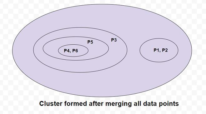
So, the final cluster can be drawn is shown as:

Hence, we have studied all three variants of the agglomerative algorithms.