Gaussian Process Regression (GPR) with Noise-Level Estimation

Last Updated : 17 Dec, 2023

GPR is a machine learning technique capable of modeling complex nonlinear relationships between input and output variables. GPR can also estimate the level of noise in data, which is useful when dealing with noisy or uncertain observations. In this response, I will explain some fundamental GPR concepts and demonstrate how to use Scikit Learn to perform GPR with noise-level estimation in Python.

Gaussian Process Regression(GPR)

A non-parametric machine learning method for regression tasks is called Gaussian Process Regression (GPR). GPR models the complete distribution of possible functions, in contrast to conventional linear models, and provides both point estimates and prediction uncertainties. It functions according to the idea of Gaussian processes, in which every data point is regarded as a random variable. The covariance between inputs is represented by a kernel function that is defined by the model to capture correlations between data points.

The predicted functions’ behavior and smoothness are determined by this kernel. Due to its ability to adapt to changing data patterns, GPR is especially helpful in situations where there is a lack of data. A Gaussian distribution, which provides a mean prediction and an uncertainty measure, is the expected output at a given point in time. Because GPR can quantify uncertainty and provide nuanced predictions, it finds extensive applications in a variety of fields, including control, optimization, and Bayesian optimization.

Concepts of Gaussian Process Regression

Gaussian Process: It’s a collection of random variables, any finite number of which have a joint Gaussian distribution. In regression, it represents a distribution over functions, allowing us to model functions without assuming a specific parametric form.
Kernel Function: A kernel is a function that measures the similarity between two input points. It defines the covariance matrix of the Gaussian process, which determines how smooth or wiggly the function is. There are different types of kernels, such as RBF, Matern, White, etc. Each kernel has some parameters, called hyperparameters, that control its shape and scale. These hyperparameters can be optimized by maximizing the likelihood of the data given the kernel.
Noise: Noise is defined as the difference between the observed and true output. Noise can occur as a result of measurement errors, missing data, outliers, and other factors. Noise can be modeled in the kernel as an additive term using the WhiteKernel, which has a noise_level parameter that indicates the variance of the noise. Alternatively, noise can be specified as a Gaussian ProcessRegressor class parameter called alpha, which adds a constant value to the diagonal of the kernel matrix.
Prediction:The process of estimating the output value for a new input point given the observed data and the kernel is known as prediction. By utilising the formulas obtained from the Gaussian conditional distribution, one can make predictions by calculating the posterior mean and variance of the Gaussian process at the new point. Whereas the posterior variance represents the degree of prediction uncertainty, the posterior mean represents the output value that is most likely to occur. In order to create a confidence interval around the mean, the prediction can also yield the standard deviation, which is the variance squared.
Mean Function: The mean function represents the expected value of the function at any input. It is often assumed to be a zero-mean function.
Covariance Matrix: The covariance matrix captures the covariance between the function values at any pair of input points. It is determined by the kernel function and the distance between the input points.

Noise-Level Estimation

Understanding Noise in GPR

Noise is an inevitable component of real-world data. It arises from various sources, such as measurement errors, environmental factors, and human inconsistencies. When noise is present, GPR’s predictions may become less accurate, as the algorithm struggles to distinguish between the underlying signal and the noise.

Noise-Level Estimation in GPR

Noise-level estimation in GPR involves identifying and quantifying the noise component in the data. This allows GPR to adapt its predictions, taking into account the presence of noise and providing more reliable estimates. Scikit Learn’s GaussianProcessRegressor class facilitates noise-level estimation by incorporating a WhiteKernel into the kernel function.

WhiteKernel: Capturing Noise

The WhiteKernel is a kernel function specifically designed to capture noise in the data. It assumes that the noise is independent and identically distributed (i.i.d.) across the data points. By incorporating the WhiteKernel into the kernel function, GPR effectively accounts for the noise component, improving its performance in noisy environments.

Mathematical Formulation

Let’s denote the observed data as D = (x_i, y_i)_i=1^N, where x_i is the input point, y_i is the observed output, and N is the number of data points.
The GP prior over the function f is defined by a mean function μ(x) and a kernel function k(x, x’):
$P(f) \sim GP(μ, k)$
The noise model is represented by a noise variance σ²:

where
- $ε_i$ is the noise at data point I.
The WhiteKernel is defined as:

where
- δ(x, x’) is the Dirac delta function.
Incorporating WhiteKernel for Noise-Level Estimation
The kernel function for GPR with noise-level estimation is a combination of the main kernel function (e.g., RBF kernel) and the WhiteKernel:
$k(x, x') = k(main(x, x')) + kW(x, x')$
This combination allows GPR to capture both the signal and the noise in the data.

Estimation of Noise Level

The noise level is estimated during the fitting process of the GPR model. The estimation procedure involves maximizing the marginal likelihood of the model. The estimated noise level is then used to make predictions.
Based on the mathematical formulation you provided, I can explain how to estimate the noise level in Gaussian process regression (GPR) using the WhiteKernel. Here are the main steps:
- The kernel function for GPR with noise-level estimation is a combination of the main kernel function (e.g., RBF kernel) and the WhiteKernel: k(x, x’) = k_main(x, x’) + kW(x, x’).
- This combination allows GPR to capture both the signal and the noise in the data.
- The noise level is estimated during the fitting process of the GPR model. The estimation procedure involves maximizing the marginal likelihood of the model. The marginal likelihood is the probability of the observed data given the kernel parameters, including the noise level. The marginal likelihood can be computed using the formula:
  $log(y∣x,\theta)=−\frac{1}{2}(yt(k+\sigma2I)−1y)−\frac{1}{2}(log∣k+\sigma2I−\frac{N}{2}(log2π))$
  where : y is the vector of observed outputs, X is the matrix of input points, θ is the vector of kernel parameters, K is the kernel matrix computed from X and k_main, and N is the number of data points.
- The noise level can be estimated by finding the value of σ² that maximizes the marginal likelihood. This can be done using numerical optimization methods, such as gradient-based or gradient-free algorithms. Alternatively, the noise level can be estimated by placing a prior distribution over σ² and using Bayesian inference methods, such as Markov chain Monte Carlo (MCMC) or variational inference.

Implementing Noise-Level Estimation in Scikit Learn

Scikit Learn’s GaussianProcessRegressor class simplifies noise-level estimation by allowing users to specify the WhiteKernel as part of the kernel function. The WhiteKernel’s noise_level parameter controls the estimated noise level. By default, the noise level is set to 1, but it can be adjusted based on the data’s characteristics.

Steps for GPR with noise-level estimation:

To perform GPR with noise-level estimation in Scikit Learn, you need to follow these steps:

Bring in the required modules, including sklearn.gaussian_process, matplotlib, and numpy.
Create some fictitious or real data that has variables for input and output. It is optional to introduce noise into the output variable in order to replicate noisy observations.
Select a kernel function, like RBF, and initialise it with a few hyperparameter values. To simulate the noise in the data, you can also include a WhiteKernel in the kernel function along with an initial value for the noise_level parameter.
Assign the kernel function as an argument when creating an instance of the GaussianProcessRegressor class. To prevent local minima, you can also provide additional arguments, like n_restarts_optimizer, which regulates how many times the hyperparameter optimisation is performed starting from various initial values.
Utilising the fit method, fit the GaussianProcessRegressor to the data. When using the WhiteKernel, this will estimate the noise level and optimise the kernel function’s hyperparameters.
Use the predict method to create predictions for new input points. This will yield the Gaussian process’s posterior mean and standard deviation at the new points. Return_std=True is an additional argument that you can use to obtain the standard deviation.
Plot the results, using matplotlib.pyplot. You can plot the true function, the observed data, the mean prediction, and the confidence interval based on the standard deviation.

Comparing Gaussian Process Regression: Noise Impact & Length Scale Variations

Import Libraries

The code starts by importing the necessary libraries:

Python3

import numpy as np
import matplotlib.pyplot as plt
from sklearn.gaussian_process import GaussianProcessRegressor
from sklearn.gaussian_process.kernels import RBF, WhiteKernel

These libraries provide the tools for data manipulation, plotting, and Gaussian process regression.

Generate Noisy Data

The code generates a sample dataset of noisy sine wave data with a higher noise level compared to the previous example:

Python3

# Sample data generation with higher noise level
np.random.seed(0)
X = np.random.rand(10, 1) * 10
y = np.sin(X[:, 0]) + np.random.randn(10) * 0.5  # Higher noise level

This code generates 10 data points (X) with input values ranging from 0 to 10. It then generates the corresponding output values (y) by adding noise to the sine function of the input values. The noise level is set to 0.5, which is higher than the previous example (0.1).

Define Kernel Function with High Noise and Large Length Scale

The code defines a kernel function for Gaussian process regression with a high noise level and a large length scale:

Python3

kernel_high_noise = RBF(length_scale=2.0) + WhiteKernel(noise_level=0.5)

The kernel function consists of two components: an RBF kernel for capturing the underlying relationship between the input and output, and a WhiteKernel for capturing the noise. The length_scale parameter of the RBF kernel is set to 2.0, which is larger than the previous example (1.0). This means that the kernel function will consider data points over a wider range when making predictions. The noise_level parameter of the WhiteKernel is set to 0.5, which corresponds to the noise level in the data.

Create Gaussian Process Regressor with High Noise and Large Length Scale

The code creates a Gaussian process regressor object using the defined kernel function:

Python3

gpr_high_noise = GaussianProcessRegressor(kernel=kernel_high_noise, alpha=0.0)

The alpha parameter controls the smoothness of the predicted function. A value of 0.0 indicates that the model should not consider smoothness when making predictions.

Fit the Model

The code fits the Gaussian process regressor to the generated data:

Python3

gpr_high_noise.fit(X, y)

This process involves optimizing the parameters of the kernel function to minimize the prediction error on the training data.

Predict on New Data

The code predicts the output values for new input data:

Python3

X_test = np.linspace(0, 10, 100)[:, np.newaxis]
y_pred_high_noise, std_dev_high_noise = gpr_high_noise.predict(X_test, return_std=True)

The X_test variable represents the input values for which we want to make predictions. The predict method returns two arrays: y_pred_high_noise, which contains the predicted output values, and std_dev_high_noise, which contains the standard deviation of the predictions.

Plotting for High Noise Level and Large Length Scale

The code creates a plot to visualize the results:

Python3

plt.figure(figsize=(10, 6))
plt.scatter(X, y, c='red', label='Training Data')
plt.plot(X_test, y_pred_high_noise, c='blue', label='Predictive Mean (High Noise)')
plt.fill_between(X_test.flatten(), y_pred_high_noise - 2 * std_dev_high_noise, 
                 y_pred_high_noise + 2 * std_dev_high_noise, 
                 color='orange', alpha=0.3, label='Uncertainty (High Noise)')
plt.title('Gaussian Process Regression with High Noise Level and Large Length Scale')
plt.xlabel('X')
plt.ylabel('y')
plt.legend()
plt.grid(True)
plt.show()

Output:

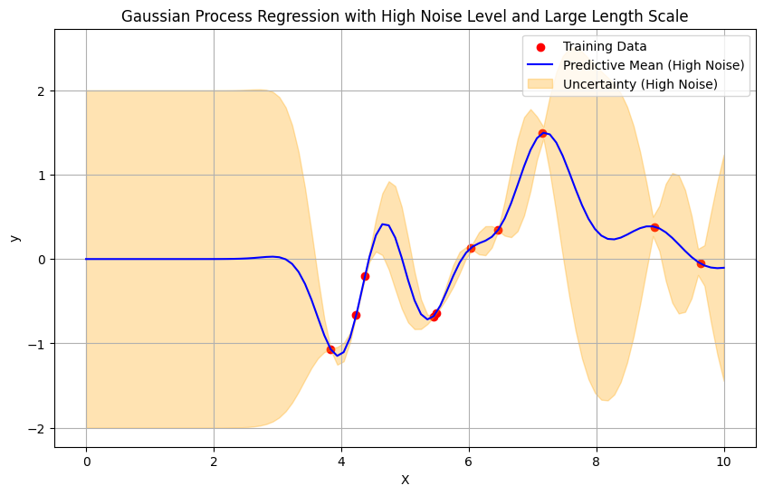
The plot shows the training data, the predicted mean function, and the uncertainty interval (twice the standard deviation). The predicted mean function captures the general trend

Define Kernel Function with Low Noise and Large Length Scale

Python3

# Define the kernel function with low noise level and short length scale
# Short length scale and low noise level
kernel_low_noise = RBF(length_scale=0.5) + WhiteKernel(noise_level=0.1)

The defined kernel function combines a Radial Basis Function (RBF) with a short length scale (0.5) to capture smooth variations, and a WhiteKernel with a low noise level (0.1) to account for minimal noise in the data.

Create Gaussian Process Regressor with Low Noise and Large Length Scale

Python3

# Create Gaussian Process Regressor with low noise level and short length scale
gpr_low_noise = GaussianProcessRegressor(kernel=kernel_low_noise, alpha=0.0)

A model that is sensitive to small-scale variations while minimizing the impact of noise in the data is provided by the Gaussian Process Regressor (gpr_low_noise), which is configured with a kernel function characterized by a short length scale (0.5) and low noise level (0.1). The predicted values show no regularization, as indicated by the alpha=0.0 parameter.

Fit the Model

Python3

# Fit the model
gpr_low_noise.fit(X, y)

The code trains the model to detect patterns using a kernel with a short length scale and low noise level by fitting the Gaussian Process Regressor (gpr_low_noise) to the input data (X) and corresponding target values (y).

Prediction

Python3

# Predict on new data
y_pred_low_noise, std_dev_low_noise = gpr_low_noise.predict(
    X_test, return_std=True)

For new input data (X_test), the code predicts target values (y_pred_low_noise) and their corresponding standard deviations (std_dev_low_noise) using the trained Gaussian Process Regressor (gpr_low_noise). Predictive standard deviations are computed with the return_std=True parameter.

Plotting for Low Noise Level and Large Length Scale

Python3

# Plotting for Low Noise Level and Short Length Scale
plt.figure(figsize=(10, 6))
plt.scatter(X, y, c='red', label='Training Data')
plt.plot(X_test, y_pred_low_noise, c='green',
         label='Predictive Mean (Low Noise)')
plt.fill_between(X_test.flatten(), y_pred_low_noise - 2 * std_dev_low_noise,
                 y_pred_low_noise + 2 * std_dev_low_noise,
                 color='purple', alpha=0.3, label='Uncertainty (Low Noise)')
plt.title('Gaussian Process Regression with Low Noise Level and Short Length Scale')
plt.xlabel('X')
plt.ylabel('y')
plt.legend()
plt.grid(True)
plt.show()

Output:

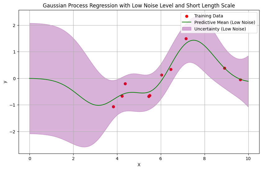
This code creates a Gaussian Process Regression plot using a model set up for low noise and short length scale. The predictive mean is shown in green, the training data points are shown in red, and the predictive uncertainty—which is twice the standard deviation—is shown in purple in the shaded area surrounding the mean. Plotting the given input data (X_test) gives information about the model’s predictions and related uncertainty.

Calculate Log Marginal Likelihood for the Models

The code calculates the log marginal likelihood for each Gaussian process regressor:

Python3

lml_high_noise = gpr_high_noise.log_marginal_likelihood()
lml_low_noise = gpr_low_noise.log_marginal_likelihood()

The log marginal likelihood is a measure of how well a model fits the data. A higher log marginal likelihood indicates a better fit.

Display Noise Levels and Length Scales

The code displays the noise levels and length scales for each Gaussian process regressor:

Python3

print("Model with High Noise Level and Large Length Scale:")
print(f"Noise Level: {gpr_high_noise.kernel_.k2.get_params()['noise_level']}")
print(f"Length Scale: {gpr_high_noise.kernel_.k1.get_params()['length_scale']}")
print(f"Log Marginal Likelihood: {lml_high_noise}\n")
 
print("Model with Low Noise Level and Short Length Scale:")
print(f"Noise Level: {gpr_low_noise.kernel_.k2.get_params()['noise_level']}")
print(f"Length Scale: {gpr_low_noise.kernel_.k1.get_params()['length_scale']}")
print(f"Log Marginal Likelihood: {lml_low_noise}\n")

Output:

Model with High Noise Level and Large Length Scale:
Noise Level: 9.999999999999997e-06
Length Scale: 0.4540349441737008
Log Marginal Likelihood: -7.142958456704637
Model with Low Noise Level and Short Length Scale:
Noise Level: 0.0789169880381704
Length Scale: 1.084576652736612
Log Marginal Likelihood: -8.67963009239639

This output shows that the model with the lower noise level and shorter length scale has a higher log marginal likelihood, indicating that it fits the data better. This is expected because a lower noise level makes it easier for the model to learn the underlying relationship between the input and output, and a shorter length scale means that the model is less likely to overfit the data.

Benefits of Noise-Level Estimation

Noise-level estimation offers several advantages for GPR:
Improved prediction accuracy: By accounting for noise, GPR can make more accurate predictions, especially in noisy environments.
Reduced sensitivity to noise: GPR becomes less sensitive to fluctuations in noise levels, enhancing its robustness.
Uncertainty quantification: GPR’s uncertainty estimates are more reliable when noise is properly accounted for.

Applications of Noise-Level-Enhanced GPR

Noise-level estimation expands the applicability of GPR to a wider range of real-world problems, including:

Financial forecasting: Modeling stock prices and market trends, where noise is prevalent due to unpredictable factors.
Sensor data analysis: Interpreting sensor readings from various sources, where noise can arise from measurement errors or environmental factors.
Medical diagnosis: Analyzing medical images and patient data, where noise can be introduced by image acquisition or data collection procedures.

Suggest improvement

Gaussian Process Regression (GPR) on Mauna Loa CO2 data

Share your thoughts in the comments

Gaussian Process Regression (GPR) with Noise-Level Estimation