Simple 1D Kernel Density Estimation in Scikit Learn

In this article, we will learn how to use Scikit learn for generating simple 1D kernel density estimation. We will first understand what is kernel density estimation and then we will look into its implementation in Python using KernelDensity class of sklearn.neighbors in scikit learn library.

Kernel density estimation

A non-parametric method for estimating the probability density function of a continuous random variable using kernels as weights is known as kernel density estimation (or KDE). It is used in a variety of tasks, like data visualization, data analysis, and machine learning. The idea behind KDE is to treat each observation point as a small probability distribution, and the density estimate is obtained by aggregating these distributions.

A kernel function is employed in KDE to estimate the density at each data point, and the separate kernel estimates are then added together to provide the final density estimate. The predicted density’s shape is determined by the kernel function, a symmetric, smooth function that is typically bell-shaped.

The formula for KDE can be expressed as follows:

Where:

• KDE(x) is the estimated density at point x.
• n is the number of data points.
• h is the bandwidth, which controls the smoothness of the estimated density.
• x_i represents each data point in the dataset.
• K(x;h) is the kernel function, which determines the contribution of each data point to the estimated density.

Some of the Commonly used kernel functions include:

1. Gaussian (or Normal) Kernel: K(x,h) = \frac{1}{\sqrt{2\pi}}\exp\left[\frac{(x-x_i)^2}{2h^2}\right]
2. Tophat Kernel: K(x;h) = \frac{1}{\sqrt{2\pi}}\exp\left(\frac{1}{2}\left|\frac{x-x_i}{h}\right|\right)
3. Epanechnikov Kernel: K(x;h) = \left[\frac{3}{4}\left(1 – (\frac{x – x_i}{h})^2   (|\frac{x – x_i}{h}| \leq 1\right)\right]
4. Exponential Kernel: K(x;h) = 0.5 \exp(-|\frac{x-x_i}{h}|)
5. Linear Kernel:
6. Cosine Kernel: K(x;h) = \frac{\pi}{4}\cos( \frac{\pi}{2}\left(\frac{x-x_i}{h}\right)) (|\frac{x-x_i}{h}| \leq 1)

The kernels used in KDE are smooth, symmetric, and usually, bell-shaped functions, and the type of kernel and width of the kernel (bandwidth) determines the smoothness and accuracy of the estimated density. The estimated density at a particular point is obtained by calculating the weighted average of the kernel functions centered at each data point, with the weights determined by the distance between the point of interest and the data points.

Code Implementation

To implement this we will first import the required libraries.

Python3

import numpy as np
import matplotlib.pyplot as plt
from sklearn.neighbors import KernelDensity

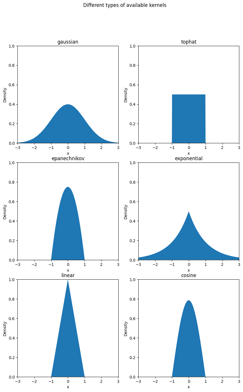
Now, we will look into different kernels available to use in this library.

Python3

# Different types of available kernels
kernels = ["gaussian", "tophat", "epanechnikov", "exponential", "linear", "cosine"]

# Create a figure with 3 rows and 2 columns
fig, ax = plt.subplots(3, 2)

# Set the size of the figure
fig.set_figheight(15)
fig.set_figwidth(10)

# Set the title of the figure
fig.suptitle("Different types of available kernels")


# Create a 1D array of x values to plot the distribution curve
x_plot = np.linspace(-6, 6, 1000)[:, np.newaxis]
x_src = np.zeros((1, 1))

# Plot the distribution curve of each kernel
for i, kernel in enumerate(kernels):
    # Calculating the log of the probability density function
    log_dens = KernelDensity(kernel=kernel).fit(x_src).score_samples(x_plot)

    # Plot the distribution curve
    ax[i // 2, i % 2].fill(x_plot[:, 0], np.exp(log_dens))

    # Set the title, x and y labels of the plot
    ax[i // 2, i % 2].set_title(kernel)
    ax[i // 2, i % 2].set_xlim(-3, 3)
    ax[i // 2, i % 2].set_ylim(0, 1)
    ax[i // 2, i % 2].set_ylabel("Density")
    ax[i // 2, i % 2].set_xlabel("x")

# Display the plot
plt.show()

Output:

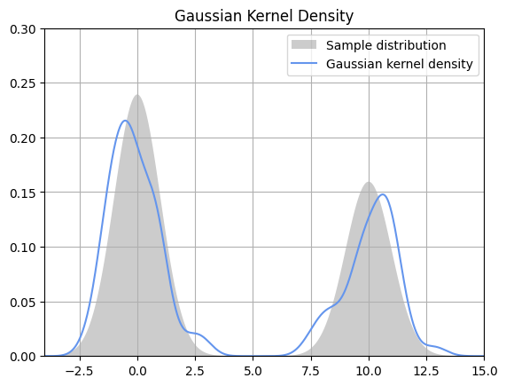
Now, let us implement kernel density estimation on random data using a Gaussian kernel with a bandwidth of 0.5.

Python3

# Plot the 1D density curve for the gaussian kernel

# Create a sample distribution
N = 100
X = np.concatenate((np.random.normal(0, 1, int(0.6 * N)),
                    np.random.normal(10, 1, int(0.4 * N)))
                )[:, np.newaxis]
X_plot = np.linspace(-5, 15, 1000)[:, np.newaxis]

# Calculate the true density
true_density = 0.6 * norm(0, 1).pdf(X_plot[:, 0]) + \
               0.4 * norm(10, 1).pdf(X_plot[:, 0])

# Creating a figure
fig, ax = plt.subplots()

# Plotting the true density
ax.fill(
    X_plot[:, 0], true_density,
    fc='black', alpha=0.2,
    label='Sample distribution'
)

# Calculating the density using the gaussian kernel with bandwidth 0.5
kde = KernelDensity(kernel='gaussian', bandwidth=0.5).fit(X)

# Calculating the log of the probability density function
log_dens = kde.score_samples(X_plot)

# Plotting the density curve
ax.plot(
    X_plot[:, 0],
    np.exp(log_dens),
    color="cornflowerblue",
    linestyle="-",
    label="Gaussian kernel density"
)

# Set the title, x and y labels of the plot
ax.set_title("Gaussian Kernel Density")
ax.set_xlim(-4, 15)
ax.set_ylim(0, 0.3)
ax.grid(True)
ax.legend(loc='upper right')

# Display the plot
plt.show()

Output: