Max Flow Problem Introduction
Last Updated :
23 Apr, 2024
The max flow problem is a classic optimization problem in graph theory that involves finding the maximum amount of flow that can be sent through a network of pipes, channels, or other pathways, subject to capacity constraints. The problem can be used to model a wide variety of real-world situations, such as transportation systems, communication networks, and resource allocation.
In the max flow problem, we have a directed graph with a source node s and a sink node t, and each edge has a capacity that represents the maximum amount of flow that can be sent through it. The goal is to find the maximum amount of flow that can be sent from s to t, while respecting the capacity constraints on the edges.
One common approach to solving the max flow problem is the Ford-Fulkerson algorithm, which is based on the idea of augmenting paths. The algorithm starts with an initial flow of zero, and iteratively finds a path from s to t that has available capacity, and then increases the flow along that path by the maximum amount possible. This process continues until no more augmenting paths can be found.
Another popular algorithm for solving the max flow problem is the Edmonds-Karp algorithm, which is a variant of the Ford-Fulkerson algorithm that uses breadth-first search to find augmenting paths, and thus can be more efficient in some cases.
Advantages:
- The max flow problem is a flexible and powerful modeling tool that can be used to represent a wide variety of real-world situations.
- The Ford-Fulkerson and Edmonds-Karp algorithms are both guaranteed to find the maximum flow in a graph, and can be implemented efficiently for most practical cases.
- The max flow problem has many interesting theoretical properties and connections to other areas of mathematics, such as linear programming and combinatorial optimization.
Disadvantages:
- In some cases, the max flow problem can be difficult to solve efficiently, especially if the graph is very large or has complex capacity constraints.
- The max flow problem may not always provide a unique or globally optimal solution, depending on the specific problem instance and algorithm used.
Maximum flow problems involve finding a feasible flow through a single-source, single-sink flow network that is maximum. Let’s take an image to explain how the above definition wants to say.
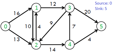
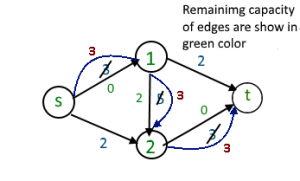
Each edge is labeled with capacity, the maximum amount of stuff that it can carry. The goal is to figure out how much stuff can be pushed from the vertex s(source) to the vertex t(sink).
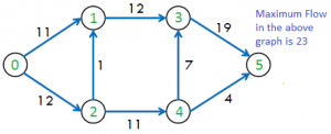
maximum flow possible is : 23
Following are different approaches to solve the problem :
1. Naive Greedy Algorithm Approach (May not produce an optimal or correct result) Greedy approach to the maximum flow problem is to start with the all-zero flow and greedily produce flows with ever-higher value. The natural way to proceed from one to the next is to send more flow on some path from s to t How Greedy approach work to find the maximum flow :
E number of edge
f(e) flow of edge
C(e) capacity of edge

1) Initialize : max_flow = 0
                f(e) = 0 for every edge 'e' in E

2) Repeat search for an s-t path P while it exists.
   a) Find if there is a path from s to t using BFS
      or DFS. A path exists if f(e) < C(e) for
      every edge e on the path.
   b) If no path found, return max_flow.
   c) Else find minimum edge value for path P

      // Our flow is limited by least remaining
      // capacity edge on path P.
      (i) flow = min(C(e)- f(e)) for path P ]
             max_flow += flow
      (ii) For all edge e of path increment flow
             f(e) += flow

3) Return max_flow
Note that the path search just needs to determine whether or not there is an s-t path in the subgraph of edges e with f(e) < C(e). This is easily done in linear time using BFS or DFS.
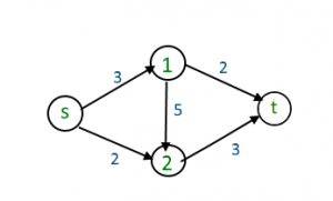
There is a path from source (s) to sink(t) [ s -> 1 -> 2 -> t] with maximum flow 3 unit ( path show in blue color ) 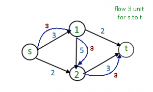
After removing all useless edge from graph it’s look like
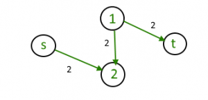
For above graph there is no path from source to sink so maximum flow : 3 unit But maximum flow is 5 unit. to over come from this issue we use residual Graph.
Below are the programs to implement the above concept:
C++
#include <iostream>
#include <limits.h>
#include <string.h>
#include <queue>

using namespace std;

// Number of vertices in given graph
#define V 6

/* Returns true if there is a path from source 's' to sink 't' in
  residual graph. Also fills parent[] to store the path */
bool bfs(int rGraph[V][V], int s, int t, int parent[])
{
    // Create a visited array and mark all vertices as not visited
    bool visited[V];
    memset(visited, 0, sizeof(visited));

    // Create a queue, enqueue source vertex and mark source vertex
    // as visited
    queue <int> q;
    q.push(s);
    visited[s] = true;
    parent[s] = -1;

    // Standard BFS Loop
    while (!q.empty())
    {
        int u = q.front();
        q.pop();

        for (int v=0; v<V; v++)
        {
            if (visited[v]==false && rGraph[u][v] > 0)
            {
                q.push(v);
                parent[v] = u;
                visited[v] = true;
            }
        }
    }

    // If we reached sink in BFS starting from source, then return
    // true, else false
    return (visited[t] == true);
}

// Returns the maximum flow from s to t in the given graph
int fordFulkerson(int graph[V][V], int s, int t)
{
    int u, v;

    // Create a residual graph and fill the residual graph with
    // given capacities in the original graph as residual capacities
    // in residual graph
    int rGraph[V][V]; // Residual graph where rGraph[i][j] indicates
                      // residual capacity of edge i-j
    for (u = 0; u < V; u++)
        for (v = 0; v < V; v++)
             rGraph[u][v] = graph[u][v];

    int parent[V];  // This array is filled by BFS and to store path

    int max_flow = 0;  // There is no flow initially

    // Augment the flow while there is path from source to sink
    while (bfs(rGraph, s, t, parent))
    {
        // Find minimum residual capacity of the edges along the
        // path filled by BFS. Or we can say find the maximum flow
        // through the path found.
        int path_flow = INT_MAX;
        for (v=t; v!=s; v=parent[v])
        {
            u = parent[v];
            path_flow = min(path_flow, rGraph[u][v]);
        }

        // update residual capacities of the edges and reverse edges
        // along the path
        for (v=t; v != s; v=parent[v])
        {
            u = parent[v];
            rGraph[u][v] -= path_flow;
            rGraph[v][u] += path_flow;
        }

        // Add path flow to overall flow
        max_flow += path_flow;
    }

    // Return the overall flow
    return max_flow;
}

// Driver program to test above functions
int main()
{
  /*
    The graph is represented as follows:

    (0) --16--> (1) --12--> (3) --20--> (5)
     |           |           |           ^
     |13         |10         |9          |
     v           v           v           |
    (2) --14--> (4) --4-->  (5) <-------|
*/

    int graph[V][V] = { {0, 16, 13, 0, 0, 0},
                        {0, 0, 10, 12, 0, 0},
                        {0, 4, 0, 0, 14, 0},
                        {0, 0, 9, 0, 0, 20},
                        {0, 0, 0, 7, 0, 4},
                        {0, 0, 0, 0, 0, 0}
                      };

    cout << "The maximum possible flow is " << fordFulkerson(graph, 0, 5);

    return 0;
}
import java.util.LinkedList;
import java.util.Queue;

public class FordFulkerson {
    static final int V = 6;

    boolean bfs(int rGraph[][], int s, int t, int parent[]) {
        boolean visited[] = new boolean[V];
        for (int i = 0; i < V; ++i)
            visited[i] = false;

        Queue<Integer> queue = new LinkedList<>();
        queue.add(s);
        visited[s] = true;
        parent[s] = -1;

        while (!queue.isEmpty()) {
            int u = queue.poll();

            for (int v = 0; v < V; v++) {
                if (!visited[v] && rGraph[u][v] > 0) {
                    queue.add(v);
                    parent[v] = u;
                    visited[v] = true;
                }
            }
        }

        return visited[t];
    }

    int fordFulkerson(int graph[][], int s, int t) {
        int u, v;
        int rGraph[][] = new int[V][V];

        for (u = 0; u < V; u++)
            for (v = 0; v < V; v++)
                rGraph[u][v] = graph[u][v];

        int parent[] = new int[V];

        int max_flow = 0;

        while (bfs(rGraph, s, t, parent)) {
            int path_flow = Integer.MAX_VALUE;
            for (v = t; v != s; v = parent[v]) {
                u = parent[v];
                path_flow = Math.min(path_flow, rGraph[u][v]);
            }

            for (v = t; v != s; v = parent[v]) {
                u = parent[v];
                rGraph[u][v] -= path_flow;
                rGraph[v][u] += path_flow;
            }

            max_flow += path_flow;
        }

        return max_flow;
    }

    public static void main(String[] args) {
        int graph[][] = { {0, 16, 13, 0, 0, 0},
                          {0, 0, 10, 12, 0, 0},
                          {0, 4, 0, 0, 14, 0},
                          {0, 0, 9, 0, 0, 20},
                          {0, 0, 0, 7, 0, 4},
                          {0, 0, 0, 0, 0, 0}
                        };
        FordFulkerson m = new FordFulkerson();

        System.out.println("The maximum possible flow is " + m.fordFulkerson(graph, 0, 5));
    }
}
from collections import deque

# Number of vertices in the given graph
V = 6

# Returns True if there is a path from source 's' to sink 't' in
# residual graph. Also fills parent[] to store the path
def bfs(rGraph, s, t, parent):
    # Create a visited array and mark all vertices as not visited
    visited = [False] * V

    # Create a queue, enqueue source vertex and mark source vertex
    # as visited
    q = deque()
    q.append(s)
    visited[s] = True
    parent[s] = -1

    # Standard BFS Loop
    while q:
        u = q.popleft()
        for v in range(V):
            if visited[v] == False and rGraph[u][v] > 0:
                q.append(v)
                parent[v] = u
                visited[v] = True

    # If we reached sink in BFS starting from source, then return
    # True, else False
    return visited[t]

# Returns the maximum flow from s to t in the given graph
def fordFulkerson(graph, s, t):
    rGraph = [[0] * V for _ in range(V)]
    for u in range(V):
        for v in range(V):
            rGraph[u][v] = graph[u][v]

    parent = [-1] * V
    max_flow = 0

    # Augment the flow while there is a path from source to sink
    while bfs(rGraph, s, t, parent):
        path_flow = float('inf')
        v = t
        while v != s:
            u = parent[v]
            path_flow = min(path_flow, rGraph[u][v])
            v = parent[v]

        v = t
        while v != s:
            u = parent[v]
            rGraph[u][v] -= path_flow
            rGraph[v][u] += path_flow
            v = parent[v]

        max_flow += path_flow

    # Return the overall flow
    return max_flow

# Driver program to test above functions
if __name__ == "__main__":
    graph = [[0, 16, 13, 0, 0, 0],
             [0, 0, 10, 12, 0, 0],
             [0, 4, 0, 0, 14, 0],
             [0, 0, 9, 0, 0, 20],
             [0, 0, 0, 7, 0, 4],
             [0, 0, 0, 0, 0, 0]]

    print("The maximum possible flow is", fordFulkerson(graph, 0, 5))
// Returns true if there is a path from source 's' to sink 't' in
// residual graph. Also fills parent[] to store the path
function bfs(rGraph, s, t, parent) {
    const visited = new Array(V).fill(false);
    const queue = [];
    queue.push(s);
    visited[s] = true;
    parent[s] = -1;

    while (queue.length !== 0) {
        const u = queue.shift();

        for (let v = 0; v < V; v++) {
            if (!visited[v] && rGraph[u][v] > 0) {
                queue.push(v);
                parent[v] = u;
                visited[v] = true;
            }
        }
    }

    return visited[t];
}

// Returns the maximum flow from s to t in the given graph
function fordFulkerson(graph, s, t) {
    const rGraph = [];
    for (let u = 0; u < V; u++) {
        rGraph[u] = new Array(V);
        for (let v = 0; v < V; v++) {
            rGraph[u][v] = graph[u][v];
        }
    }

    const parent = new Array(V);
    let max_flow = 0;

    while (bfs(rGraph, s, t, parent)) {
        let path_flow = Number.MAX_VALUE;
        for (let v = t; v !== s; v = parent[v]) {
            const u = parent[v];
            path_flow = Math.min(path_flow, rGraph[u][v]);
        }

        for (let v = t; v !== s; v = parent[v]) {
            const u = parent[v];
            rGraph[u][v] -= path_flow;
            rGraph[v][u] += path_flow;
        }

        max_flow += path_flow;
    }

    return max_flow;
}

// Driver code
const V = 6;
const graph = [
    [0, 16, 13, 0, 0, 0],
    [0, 0, 10, 12, 0, 0],
    [0, 4, 0, 0, 14, 0],
    [0, 0, 9, 0, 0, 20],
    [0, 0, 0, 7, 0, 4],
    [0, 0, 0, 0, 0, 0]
];

console.log("The maximum possible flow is " + fordFulkerson(graph, 0, 5));
OutputThe maximum possible flow is 23
2. Residual Graphs
The idea is to extend the naive greedy algorithm by allowing “undo” operations. For example, from the point where this algorithm gets stuck in above image, we’d like to route two more units of flow along the edge (s, 2), then backward along the edge (1, 2), undoing 2 of the 3 units we routed the previous iteration, and finally along the edge (1,t) 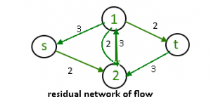
backward edge : ( f(e) ) and forward edge : ( C(e) – f(e) ) We need a way of formally specifying the allowable “undo” operations. This motivates the following simple but important definition, of a residual network. The idea is that, given a graph G and a flow f in it, we form a new flow network Gf that has the same vertex set of G and that has two edges for each edge of G. An edge e = (1,2) of G that carries flow f(e) and has capacity C(e) (for above image ) spawns a “forward edge” of Gf with capacity C(e)-f(e) (the room remaining) and a “backward edge” (2,1) of Gf with capacity f(e) (the amount of previously routed flow that can be undone). source(s)- sink(t) paths with f(e) < C(e) for all edges, as searched for by the naive greedy algorithm, corresponding to the special case of s-t paths of Gf that comprise only forward edges.
The idea of residual graph is used The Ford-Fulkerson and Dinic’s algorithms
Source : http://theory.stanford.edu/~tim/w16/l/l1.pdf
Share your thoughts in the comments
Please Login to comment...