Composite Transformation in 2-D graphics

Prerequisite – Basic types of 2-D Transformation :

1. Translation
2. Scaling
3. Rotation
4. Reflection
5. Shearing of a 2-D object

Composite Transformation :
As the name suggests itself Composition, here we combine two or more transformations into one single transformation that is equivalent to the transformations that are performed one after one over a 2-D object. 

Example :
Consider we have a 2-D object on which we first apply transformation T₁ (2-D matrix condition) and then we apply transformation T₂(2-D matrix condition) over the 2-D object and the object get transformed, the very equivalent effect over the 2-D object we can obtain by multiplying T₁ & T₂ (2-D matrix conditions) with each other and then applying the T₁₂ (resultant of T₁ X T₂) with the coordinates of the 2-D image to get the transformed final image. 

Problem :
Consider we have a square O(0, 0), B(4, 0), C(4, 4), D(0, 4) on which we first apply T1(scaling transformation) given scaling factor is Sx=Sy=0.5 and then we apply T2(rotation transformation in clockwise direction) it by 90^*(angle), in last we perform T3(reflection transformation about origin).

Ans : The square O, B, C, D looks like : 

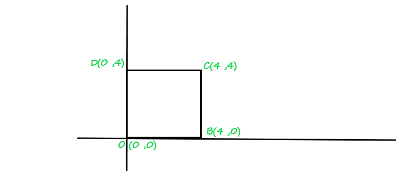
Square_given(Fig.1)

First, we perform scaling transformation over a 2-D object :

Representation of scaling condition :

[Tex]\begin{bmatrix}x'\\y'\end{bmatrix}=\begin{bmatrix}Sx&0\\0&Sx\end{bmatrix}*\begin{bmatrix}x\\y\end{bmatrix}\\[/Tex]

For coordinate O(0, 0) :
[Tex]O\begin{bmatrix}x\\y\end{bmatrix}=\begin{bmatrix}0.5&0\\0&0.5\end{bmatrix}*\begin{bmatrix}0\\0\end{bmatrix}\\\\[1ex]O\begin{bmatrix}\\x’\\y’\end{bmatrix}=\begin{bmatrix}0\\0\end{bmatrix}  [/Tex]

For coordinate B(4, 0) :
[Tex]B\begin{bmatrix}x\\y\end{bmatrix}=\begin{bmatrix}0.5&0\\0&0.5\end{bmatrix}*\begin{bmatrix}4\\0\end{bmatrix}\\\\[1ex]B\begin{bmatrix}\\x’\\y’\end{bmatrix}=\begin{bmatrix}2\\0\end{bmatrix}  [/Tex]

For coordinate C(4, 4) :
[Tex]C\begin{bmatrix}x\\y\end{bmatrix}=\begin{bmatrix}0.5&0\\0&0.5\end{bmatrix}*\begin{bmatrix}4\\4\end{bmatrix}\\\\[1ex]C\begin{bmatrix}\\x’\\y’\end{bmatrix}=\begin{bmatrix}2\\2\end{bmatrix}  [/Tex]

For coordinate D(0, 4) :
[Tex]D\begin{bmatrix}x\\y\end{bmatrix}=\begin{bmatrix}0.5&0\\0&0.5\end{bmatrix}*\begin{bmatrix}0\\4\end{bmatrix}\\\\[1ex]D\begin{bmatrix}\\x’\\y’\end{bmatrix}=\begin{bmatrix}0\\2\end{bmatrix}  [/Tex]

2-D object after scaling :

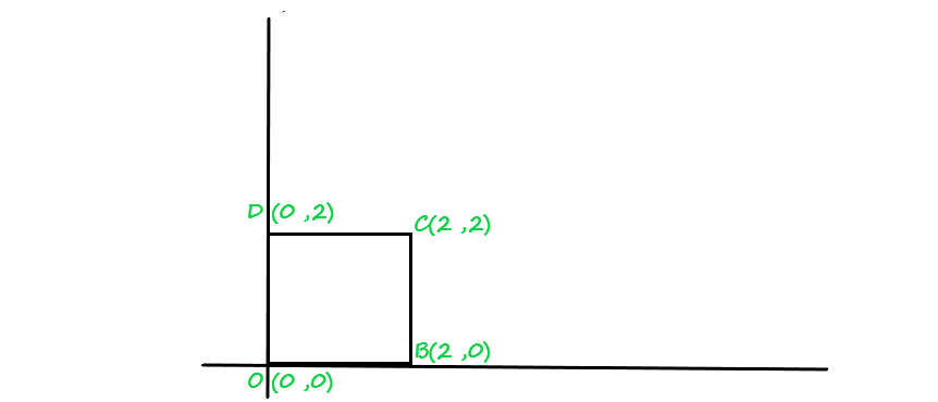
Fig.2

*Now, we’ll perform rotation transformation in clockwise-direction on Fig.2 by 90^θ:

The condition of rotation transformation of 2-D object about origin is :

[Tex]\begin{bmatrix}x'\\y'\end{bmatrix}=\begin{bmatrix}cosθ&sinθ\\-sinθ&cosθ\end{bmatrix}*\begin{bmatrix}x\\y\end{bmatrix}\\\\[1ex] Cos90 = 0 \\ sin90=1[/Tex]

For coordinate O(0, 0) :
[Tex]O\begin{bmatrix}x’\\y’\end{bmatrix}=\begin{bmatrix}0&1\\-1&0\end{bmatrix}*\begin{bmatrix}0\\0\end{bmatrix}\\\\[1ex]O\begin{bmatrix}\\x’\\y’\end{bmatrix}=\begin{bmatrix}0\\0\end{bmatrix}  [/Tex]

For coordinate B(2, 0) :
[Tex]B\begin{bmatrix}x’\\y’\end{bmatrix}=\begin{bmatrix}0&1\\-1&0\end{bmatrix}*\begin{bmatrix}2\\0\end{bmatrix}\\\\[1ex]B\begin{bmatrix}\\x’\\y’\end{bmatrix}=\begin{bmatrix}0\\-2\end{bmatrix}  [/Tex]

For coordinate C(2, 2) :
[Tex]C\begin{bmatrix}x’\\y’\end{bmatrix}=\begin{bmatrix}0&1\\-1&0\end{bmatrix}*\begin{bmatrix}2\\2\end{bmatrix}\\\\[1ex]C\begin{bmatrix}\\x’\\y’\end{bmatrix}=\begin{bmatrix}2\\-2\end{bmatrix}  [/Tex]

For coordinate D(0, 2) :
[Tex]D\begin{bmatrix}x’\\y’\end{bmatrix}=\begin{bmatrix}0&1\\-1&0\end{bmatrix}*\begin{bmatrix}0\\2\end{bmatrix}\\\\[1ex]D\begin{bmatrix}\\x’\\y’\end{bmatrix}=\begin{bmatrix}2\\0\end{bmatrix}  [/Tex]

2-D object after rotating about origin by 90^* angle :

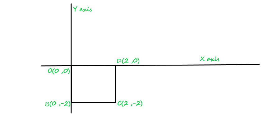
Fig.3

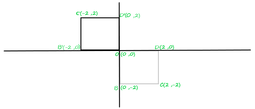
*Now, we’ll perform third last operation on Fig.3, by reflecting it about origin :

The condition of reflecting an object about origin is 

[Tex]\begin{bmatrix}x'\\y'\end{bmatrix}=\begin{bmatrix}-1&0\\0&-1\end{bmatrix}*\begin{bmatrix}x\\y\end{bmatrix}\\\\[1ex][/Tex]

For coordinate O(0, 0) :
[Tex]O\begin{bmatrix}x’\\y’\end{bmatrix}=\begin{bmatrix}-1&0\\0&-1\end{bmatrix}*\begin{bmatrix}0\\0\end{bmatrix}\\\\[1ex]O\begin{bmatrix}\\x’\\y’\end{bmatrix}=\begin{bmatrix}0\\0\end{bmatrix}  [/Tex]

For coordinate B'(0, 0) :
[Tex]B’\begin{bmatrix}x’\\y’\end{bmatrix}=\begin{bmatrix}0&-1\\-1&0\end{bmatrix}*\begin{bmatrix}0\\2\end{bmatrix}\\\\[1ex]B’\begin{bmatrix}\\x’\\y’\end{bmatrix}=\begin{bmatrix}-2\\0\end{bmatrix}  [/Tex]

For coordinate C'(0, 0) :
[Tex]C’\begin{bmatrix}x’\\y’\end{bmatrix}=\begin{bmatrix}-1&0\\0&-1\end{bmatrix}*\begin{bmatrix}2\\-2\end{bmatrix}\\\\[1ex]C’\begin{bmatrix}\\x’\\y’\end{bmatrix}=\begin{bmatrix}-2\\2\end{bmatrix}  [/Tex]

For coordinate D'(0, 0) :
[Tex]D’\begin{bmatrix}x’\\y’\end{bmatrix}=\begin{bmatrix}-1&0\\0&-1\end{bmatrix}*\begin{bmatrix}0\\-2\end{bmatrix}\\\\[1ex]D’\begin{bmatrix}\\x’\\y’\end{bmatrix}=\begin{bmatrix}0\\2\end{bmatrix}  [/Tex]

The final 2-D object after reflecting about origin, we get :

Fig.4

Note : The above finale result of Fig.4, that we get after applying all transformation one after one in a serial manner. We could also get the same result by combining all the transformation 2-D matrix conditions together and multiplying each other and get a resultant of multiplication(R). Then, applying that 2D-resultant matrix(R) at each coordinate of the given square(above). So, you will get the same result as you have in Fig.4.

Solution using Composite transformation :
*First we multiplied 2-D matrix conditions of Scaling transformation with Rotation transformation :

[Tex]\begin{bmatrix}R_1\end{bmatrix}=\begin{bmatrix}0.5&0\\0&0.5\end{bmatrix}*\begin{bmatrix}0&1\\-1&0\end{bmatrix}\\\\[1ex]\begin{bmatrix}\\R_1\end{bmatrix}=\begin{bmatrix}0&0.5\\-0.5&0\end{bmatrix}  [/Tex]

*Now, we multiplied Resultant 2-D matrix(R₁) with the third last given Reflecting condition of transformation(R₂) to get Resultant(R) : 

[Tex]\begin{bmatrix}R\end{bmatrix}=\begin{bmatrix}0&0.5\\-0.5&0\end{bmatrix}*\begin{bmatrix}-1&0\\0&-1\end{bmatrix}\\\\[1ex]\begin{bmatrix}\\R\end{bmatrix}=\begin{bmatrix}0&-0.5\\0.5&0\end{bmatrix}  [/Tex]

Now, we’ll applied the Resultant(R) of 2d-matrix at each coordinate of the given object (square) to get the final transformed or modified object. 

First transformed coordinate O(0, 0) is :
[Tex]O\begin{bmatrix}x’\\y’\end{bmatrix}=\begin{bmatrix}0&-0.5\\0.5&0\end{bmatrix}*\begin{bmatrix}0\\0\end{bmatrix}\\\\[1ex]O\begin{bmatrix}\\x’\\y’\end{bmatrix}=\begin{bmatrix}0\\0\end{bmatrix}  [/Tex]

Second, transformed coordinate B'(4, 0) is :
[Tex]B’\begin{bmatrix}x’\\y’\end{bmatrix}=\begin{bmatrix}0&-0.5\\0.5&0\end{bmatrix}*\begin{bmatrix}4\\0\end{bmatrix}\\\\[1ex]B’\begin{bmatrix}\\x’\\y’\end{bmatrix}=\begin{bmatrix}0\\2\end{bmatrix}  [/Tex]

Third transformed coordinate C'(4, 4) is :
[Tex]C’\begin{bmatrix}x’\\y’\end{bmatrix}=\begin{bmatrix}0&-0.5\\0.5&0\end{bmatrix}*\begin{bmatrix}4\\4\end{bmatrix}\\\\[1ex]C’\begin{bmatrix}\\x’\\y’\end{bmatrix}=\begin{bmatrix}-2\\2\end{bmatrix}  [/Tex]

Fourth transformed coordinate D'(0, 4) is :
[Tex]D’\begin{bmatrix}x’\\y’\end{bmatrix}=\begin{bmatrix}0&-0.5\\0.5&0\end{bmatrix}*\begin{bmatrix}0\\4\end{bmatrix}\\\\[1ex]D’\begin{bmatrix}\\x’\\y’\end{bmatrix}=\begin{bmatrix}-2\\0\end{bmatrix}  [/Tex]

The final result of the transformed object that you get would be same as above :