Calculus is a branch of mathematics that studies the properties and behavior of functions, rates of change, limits, and infinite series. Calculus has many applications in science, engineering, economics, and other fields. However, calculus can also be challenging to learn and master, especially for beginners.
That is why we have prepared this calculus cheat sheet, a handy reference guide covering the most important concepts, formulas, rules, and calculus examples. Whether you need a quick review, a study aid, or a problem solver, this cheat sheet will help you ace calculus with ease.
Read: Calculus in Maths
What is Limit?
Limit of a function f(x) as x approaches c, denoted as lim f(x)=L, exists if, for every ϵ>0, there exists a δ>0 such that for all
0 <∣x-c∣ < δ ⇒ ∣f(x)-L∣ < ϵ
Left Hand and Right Hand Limit
| Left-Hand Limit | [Tex]\lim_{x \to a^{-}}f(x)=\lim_{h \to 0^{-}}f(a-h)[/Tex] |
|---|
| Right-Hand Limit | [Tex]\lim_{x \to a^{+}}f(x)=\lim_{h \to 0^{+}}f(a+h)[/Tex] |
|---|
Existence of Limit
For Existence of [Tex]\bold{\lim_{x \to a}f(x)} [/Tex],
- [Tex]\lim_{x \to a^{-}}f(x) [/Tex]and [Tex]\lim_{x \to a^{+}}f(x) [/Tex]exists, and
- [Tex]\lim_{x \to a^{-}}f(x) = \lim_{x \to a^{+}}f(x)[/Tex]
Properties of Limits
Common properties of Limits are:
| [Tex]\lim _{x \rightarrow a}[f(x) \pm g(x)][/Tex] | [Tex]\lim _{x \rightarrow a} f(x) \pm \lim _{x \rightarrow a} g(x)[/Tex] |
| [Tex]\lim _{x \rightarrow a}[k f(x)][/Tex] | [Tex]k \lim _{x \rightarrow a} f(x),[/Tex] |
| [Tex]\lim _{x \rightarrow a}[f(x) g(x)][/Tex] | [Tex]\lim _{x \rightarrow a} f(x) \lim _{x \rightarrow a} g(x)[/Tex] |
| [Tex]\lim _{x \rightarrow a} \frac{f(x)}{g(x)}[/Tex] | [Tex]\frac{\lim _{x \rightarrow a} f(x)}{\lim _{x \rightarrow a} g(x)}, [/Tex]provided [Tex]\lim _{x \rightarrow a} g(x) \neq 0[/Tex] |
| [Tex]\lim _{x \rightarrow a}[f(x)]^{g(x)}[/Tex] | [Tex]\left[\lim _{x \rightarrow a} f(x)\right]^{\lim _{x \rightarrow a} g(x)}[/Tex] |
| [Tex]\lim _{x \rightarrow a}(g \circ f)(x)[/Tex] | [Tex]\lim _{x \rightarrow a} g[f(x)]=g\left[\lim _{x \rightarrow a} f(x)\right][/Tex] |
| [Tex]\lim _{x \rightarrow a} \log f(x)[/Tex] | [Tex]\log \left[\lim _{x \rightarrow a} f(x)\right], [/Tex]provided [Tex]\lim _{x \rightarrow a} f(x)>0.[/Tex] |
| [Tex]\lim _{x \rightarrow a} e^{f(x)}[/Tex] | [Tex]e^{\lim _{x \rightarrow a} f(x)}[/Tex] |
| [Tex]\lim _{x \rightarrow a}|f(x)|[/Tex] | [Tex]\left|\lim _{x \rightarrow a} f(x)\right|[/Tex] |
| [Tex]\lim _{x \rightarrow a} f(x)=+\infty \ or -\infty[/Tex] | [Tex]\lim _{x \rightarrow a} \frac{1}{f(x)}=0[/Tex] |
Some important formulas for limits are:
| [Tex]\lim _{x \rightarrow a} \frac{x^n-a^n}{x-a}[/Tex] | [Tex]n a^{n-1}, n \in Q[/Tex] |
| [Tex]\lim _{x \rightarrow 0} \frac{(1+x)^n-1}{x}[/Tex] | [Tex]n, n \in Q[/Tex] |
| [Tex]\lim _{x \rightarrow 0} \frac{\sin x}{x}=\lim _{x \rightarrow 0} \frac{x}{\sin x}[/Tex] | 1 |
| [Tex]\lim _{x \rightarrow 0} \frac{\tan x}{x}=\lim _{x \rightarrow 0} \frac{x}{\tan x}[/Tex] | 1 |
| [Tex]\lim _{x \rightarrow 0} \frac{\sin ^{-1} x}{x}=\lim _{x \rightarrow 0} \frac{x}{\sin ^{-1} x}[/Tex] | 1 |
| [Tex]\lim _{x \rightarrow 0} \frac{\tan ^{-1} x}{x}=\lim _{x \rightarrow 0} \frac{x}{\tan ^{-1} x}[/Tex] | 1 |
| [Tex]\lim _{x \rightarrow 0} \frac{\sin x^{\circ}}{x}[/Tex] | [Tex]\frac{\pi}{180}[/Tex] |
| [Tex]\lim _{x \rightarrow 0} \cos x[/Tex] | 1 |
| [Tex]\lim _{x \rightarrow a} \frac{\sin (x-a)}{x-a}[/Tex] | 1 |
| [Tex]\lim _{x \rightarrow a} \frac{\tan (x-a)}{x-a}[/Tex] | 1 |
| [Tex]\lim _{x \rightarrow a} \sin ^{-1} x[/Tex] | [Tex]\sin ^{-1} a,|a| \leq 1[/Tex] |
| [Tex]\lim _{x \rightarrow a} \cos ^{-1} x[/Tex] | [Tex]\cos ^{-1} a,|a| \leq 1[/Tex] |
| [Tex]\lim _{x \rightarrow a} \tan ^{-1} x[/Tex] | [Tex]\tan ^{-1} a,-\infty<a<\infty[/Tex] |
| [Tex]\lim _{x \rightarrow \infty} \frac{\sin x}{x}=\lim _{x \rightarrow \infty} \frac{\cos x}{x}[/Tex] | 0 |
| [Tex]\lim _{x \rightarrow \infty} \frac{\sin \frac{1}{x}}{\frac{1}{x}}[/Tex] | 1 |
| [Tex]\lim _{x \rightarrow 0} \frac{1-\cos x}{x}[/Tex] | 0 |
| [Tex]\lim _{x \rightarrow 0} \frac{e^x-1}{x}[/Tex] | 1 |
| [Tex]\lim _{x \rightarrow 0} \frac{a^x-1}{x}[/Tex] | [Tex]\log _e a, a>0[/Tex] |
| [Tex]\lim _{x \rightarrow 0} \frac{\log _e(1+x)}{x}[/Tex] | 1 |
| [Tex]\lim _{x \rightarrow e} \log _e x[/Tex] | -1 |
| [Tex]\lim _{x \rightarrow 0} \frac{\log _a(1+x)}{x}[/Tex] | [Tex]\log _a e, a>0, \neq 1[/Tex] |
Learn More Limit Formulas.
Evaluation of Limits
There are various methods for evaluation of limits such as:
Substitution: This is the simplest method, where we just plug in the value of the limit into the function and see if it works. For example,
lim x → 2 x2 + 3x − 4 = (2)2 + 3(2) – 4 = 4 + 6 – 4 = 6.
Factoring: This method is helpful when substitution gives us an indeterminate form, such as 0/0 or 10, where k is a constant. In this case, we can try to factor the numerator and denominator of the function and cancel out any common factors. For example, limx → 2 (x2 – 4)/(x − 2). If we substitute x = 2 here, limit becomes 0/0 form. Thus, it can be calculated as:
limx → 2 (x2 – 4)/(x − 2) = limx → 2 [(x – 2)(x + 2)]/(x − 2) = limx → 2 (x + 2) = 2 + 2 = 4
Algebraic manipulation: This method involves simplifying the function by using algebraic rules, such as expanding, combining, or dividing terms. For example,
limx → 0 (x2 + 2x)/(x2 – 2x) = limx → 0 x(x + 2)/x(x – 2) = limx → 0 (x + 2)/(x – 2) = (0 + 2)/(0 – 2) = 2/(-2) = -1.
L Hospital Rule
If limx → a f(x)/g(x) is in the form of 0/0 or ∞/∞ then
[Tex]\lim_{x \to a}\frac{f(x)}{g(x)} = \lim_{x \to a}\frac{f'(x)}{g'(x)}[/Tex]
Where f'(x) and g'(x) are the first order derivatives of functions f(x) and g(x) respectively.
Other Indeterminant forms in limits are:
Read More about L Hospital Rule.
Sandwich Theorem
For functions f(x), g(x), and h(x) such that f(x) ≤ g(x) ≤ h(x) then for some value ‘a’ if [Tex] \bold{\lim_{x \to a}f(x)} = p = \bold{\lim_{x \to a}h(x)} [/Tex]then
[Tex]\bold{\lim_{x \to a}g(x)= p}[/Tex]
Read more about Sandwich Theorem.
Continuity, Discontinuity, and Differentiability of a Function
The conditions for continuity, discontinuity, and differentiability of a function at a point are tabulated below:
| Continuity | Discontinuity | Differentiability |
|---|
| [Tex]\lim_{x \to a^{-}}f(x)=\lim_{x \to a^{+}}f(x)=f(a)[/Tex] | - f(a) not defined
- Either Left Hand Limit or Right LImit doesn’t exist or infinite
- [Tex]\lim_{x \to a^{-}}f(x)\neq\lim_{x \to a^{+}}f(x)[/Tex]
- [Tex]\lim_{x \to a^{-}}f(x)=\lim_{x \to a^{+}}f(x)\neq{f(a)}[/Tex]
| - [Tex]\lim_{x \to a}\frac{f(x)-f(a)}{x-a} [/Tex]has finite value
- If Left Hand Derivative Right Hand Derivative i.e. [Tex]\lim_{x \to a^{-}}\frac{f(x)-f(a)}{x-a}=\lim_{x \to a^{+}}\frac{f(x)-f(a)}{x-a}[/Tex]
|
Theorems of Continuity
Some common theorems related to continuity are:
- If f and g are continuous functions then f±g, fg, f/g (where, g≠0), and cf(x) all are continuous.
- If g is continuous at ‘a’ and f is continuous at g(a) then fog is also continuous at ‘a’.
- If f is continuous in its domain then |f| is also continuous in its domain
- If f is continuous in the domain D then 1/f is also continuous in D-{x:f(x) = 0}.
Fundamental Theorems of Differentiability
Some common theorems related to differentiability are:
- If f and g are two differential functions then their sum, difference, product, and quotients are also differentiable.
- If f and g are two differential functions then fog is also differentiable.
- If f and g are not differential functions then their sum and product functions can be differential functions.
Learn More Continuity and Discontinuity
Derivatives
Derivative is the rate of change of a function with respect to its inputs. The derivative of a function f(x) at a particular point x, denoted as f'(x) or df/dx(x), is equal to the slope of the tangent line to the function at that point. Derivatives can be expressed as:
| Derivative at a Point | [Tex]\bold{\lim_{x \to c}\frac{f(x)-f(c)}{x-c}}[/Tex] |
|---|
| Derivative of a Function | [Tex]\bold{f'(x) = \lim_{h \to 0} \frac{f(x + h) -f(x)}{h}}[/Tex] |
|---|
| Derivative as a Rate Measure | [Tex]\dfrac{dy}{dx}=\bold{\lim_{\Delta x \to 0}\dfrac{\Delta y}{\Delta x}}[/Tex] |
|---|
| Differentiation from the First Principle | [Tex]\bold{f'(x) = \lim_{h \to 0} \frac{f(x + h) -f(x)}{h}}[/Tex] |
|---|
Algebra of Derivatives
Algebra of derivatives refers to the rules and formulas used to find the derivative of algebraic functions. Some rules for derivatives are:
| Sum Rule | {f(x) + g(x)}’ = f'(x) + g'(x) |
|---|
| Difference Rule | {f(x) – g(x)}’ = f'(x) – g'(x) |
|---|
| Product Rule | {f(x).g(x)}’ = f'(x).g(x) + f(x).g'(x) |
|---|
| Quotient Rule | {f(x)/g(x)}’ = {f'(x).g(x) – f(x).g'(x)}/(g(x))2 |
|---|
Learn More, Algebra of Derivatives
Some of the common formulas to find derivative are:
| d/dx(c) | 0 |
| d/dx{c.f(x)} | c.f'(x) |
| d/dx(x) | 1 |
| d/dx(xn) | nxn-1 |
| d/dx{f(g(x))} | f'(g(x)).g'(x) |
| d/dx(ax) | ax.ln(a) |
| d/dx{ln(x)} {Note: ln(x) = loge(x)} | 1/x, x>0 |
| d/dx(logax) | 1/xln(a) |
| d/dx(ex) | ex |
| d/dx{sin(x)} | cos(x) |
| d/dx{cos(x)} | -sin(x) |
| d/dx{tan(x)} | sec2x |
| d/dx{sec(x)} | sec(x).tan(x) |
| d/dx{cosec(x)} | -cosec(x).cot(x) |
| d/dx{cot(x)} | -cosec2(x) |
| d/dx{sin-1(x)} | 1/√(1 – x2) |
| d/dx{cos-1(x)} | -1/√(1 – x2) |
| d/dx{tan-1(x)} | 1/(1+x2) |
Check,
Differentiation of Function of a Function
It says that if f(x) and g(x) are differentiable functions then fog is also differentiable.
d/dx{(fog)(x)} = d/dx{fog(x)}.d/dx{g(x)}
OR
y = g(x) and z = f(y), then dz/dx = (dz/dy).(dy/dx)
Differentiation Rules
Some common rules for differentiation are:
| Rule | Function, f(x) | Derivative, f'(x) |
|---|
| Constant Multiple Rule | c ⋅f(x) | c ⋅ f′(x) |
| Sum Rule | f(x) + g(x) | f′(x) + g′(x) |
| Difference Rule | f(x) − g(x) | f′(x) − g′(x) |
| Product Rule | f(x)⋅g(x) | f(x)g'(x) + f'(x)g(x) |
| Quotient Rule | g(x)f(x) | (g(x)f'(x) – f(x)g'(x)) / (g(x))2 |
| Chain Rule | f(g(x)) | f′(g(x))⋅g′(x) |
Where f'(x) represents first order derivative of f(x).
Some of the examples of chain rule are:
| d/dx[{f(x)}n] | n[{f(x)}n-1].f'(x) |
| d/dx[ln{f(x)}] | {1/f(x)}.f'(x) |
| d/dx{ef(x)} | ef(x).f'(x) |
| d/dx{sin(f(x))} | cos(f(x)).f'(x) |
| d/dx{cos(f(x))} | -sin(f(x)).f'(x) |
| d/dx{tan(f(x))} | sec2(f(x)).f'(x) |
| d/dx{tan-1(f(x))} = {1/(1+(f(x))2)}.f'(x) | {1/(1+(f(x))2)}.f'(x) |
Read More,
Differentiation of Determinant
Let’s say we have to differentiate a determinant given in terms of x, then its derivative is given as differentiation of row (or column) at a time.
If [Tex]\bold{|x| = \begin{vmatrix}f(x)&g(x) \\ u(x)&v(x)\end{vmatrix}}[/Tex]
Then [Tex]\bold{|x|’ = \begin{vmatrix}f'(x)&g'(x) \\ u(x)&v(x)\end{vmatrix} + \begin{vmatrix}f(x)&g(x) \\ u'(x)&v'(x)\end{vmatrix}}[/Tex]
Where |x|’ represents the first order derivative fo |x|.
Extreme Value Theorem
If f(x) is continuous in the closed interval [a, b] then there exists c ≥ a for which f(c) is minimum and d ≤ b for which f(d) is minimum. In short, for a ≤ c and d ≤ b, f(c) is the absolute minimum in the closed interval [a, b] and f(d) is the absolute maximum in the closed interval [a, b].
Mean Value Theorem
Mean Value Theorem states that if a function f(x) is continuous in the closed interval [a, b] and differentiable in the open interval (a, b) then there exists a point c in (a, b) such that
f'(c) = [f(b) – f(a)]/(b-a)
Learn More, Rolle’s Theorem and Lagrange’s Mean Value Theorem
Implicit Differentiation
Implicit Differentiation is used when a function is not defined explicitly in terms of only one independent variable.
Let’s say we have a function g(x, y) = x2 + y + 3xy
then g'(x, y) = d{g(x,y)}/dx = 2x + y’ + 3y + 3xy’
⇒ g'(x,y) = 2x + 3y + y'(1 + 3x).
Higher Order Derivatives
Higher Order Derivatives refer to the derivative of derivative of a function. In this, we first differentiate a function and find its derivatives and then again differentiate the derivative obtained for the first time. If differentiation is done two times then it is called Second Order Derivative and if done for ‘n’ times it is called nth order derivative. For a function defined as y = f(x), its higher-order derivatives are given as follows:
| Second Order Derivative | f”(x) = f2(x) = d2y/dx2 = {f'(x)}’ |
|---|
| nth Order Derivative | fn(x) = dny/dxn = {f(n-1)(x)}’ |
|---|
Increasing and Decreasing Function
Let f(x) is a function differentiable on (a, b) then the function is
| Increasing | f'(x) > 0 |
|---|
| Decreasing | f'(x) < 0 |
|---|
| Constant | f'(x) = 0 |
|---|
Learn More, Increasing and Decreasing Function
Critical Point
Critical Point is the point where the derivative of the function is either zero or not defined. C is the critical point of the function f(x) if
(dy/dx)x = C = 0
OR
(dy/dx)x = C = Not Defined
Concave Up and Concave Down
| Concave Up | f”(x) > 0 at x = a |
|---|
| Concave Down | f”(x) < 0 at x = a |
|---|
Inflection Point
The point at which the concavity of a function changes is called the Inflection Point. The below-mentioned steps can be used to find the inflection point:
Step 1: Find the second-order derivative of the function i.e. f”(x).
Step 2: Equate f”(x) = 0 and find x.
Step 3: Take a point smaller than x and one larger than x.
Step 4. Put the values in f”(x) and observe the sign. If the sign changes from a value lower than x to a value larger than x then an inflection point exists.
Maxima and Minima
| Absolute Maximum | x = a | f(x) ≤ f(a) where x and a belong to domain of f. |
|---|
| Absolute Minimum | x = a | f(x) ≥ f(a) where x and a belong to domain of f. |
|---|
| Local Maxima | x = a | f(x) ≤ f(a) for all x near to a. |
|---|
| Local Minima | x = a | f(x) ≥ f(a) for all x near to a. |
|---|
Learn More, Absolute Maxima and Minima and Relative Maxima and Minima
First Derivative Test
Local Minima
| Local Maxima
|
|---|
If x = a is point of local minima then
- f'(a) = 0 and
- f'(x) > 0 for points right to x = a and f'(x) < 0 for points left to x = a
| If x = a is the point of local maxima then
- f'(a) = 0 and
- f'(x) > 0 for points left to x = a and f'(x) < 0 for points right to x = a.
|
Second Derivative Test
If x = a is a critical point of f(x) such that f'(a) = 0 then if
| f”(a) < 0 | x = a is the point of local maxima |
|---|
| f”(a) > 0 | x = a is the point of local minima |
|---|
| f”(a) = 0 | x = a may be a point of local maxima or local minima or none. |
|---|
Differential Equation
Differential Equation refers to an equation that has a dependent variable, an independent variable, and a differential coefficient of the dependent variable with respect to the independent variable.
Order and Degree of Differential Equation
| Order of Differential Equation | Degree of Differential Equation |
|---|
Highest Derivative in the Equation
Example: In (dy/dx)2 + 3(d2y/dx2)3 Order is 2.
| Exponent raised to Highest Derivative
Example: In (dy/dx)3 + 3(d2y/dx2)2 Degree is 3.
|
Solution of First Order and First Degree Differential Equation
The solution of a first-order and first-degree differential equation can be found by different techniques depending upon the category they belong to.
Equation of the Standard Form
If a differential equation is in the form f[f1(x,y)]d{f1(x,y)} + Φ[f2(x,y)]d{f2(x,y)} + … = 0 then each term can be integrated separately. Some of the standard terms can be replaced by the exact differentials mentioned below:
| xdy + ydx | d(xy) |
| dx + dy | d(x + y) |
| (xdy – ydx)/x2 | d(y/x) |
| (ydx – xdy)/y2 | d(x/y) |
| (xdy + ydx)/xy | d(log xy) |
| (ydx – xdy)/xy | d(log x/y) |
| (xdy – ydx)/xy | d(log y/x) |
| (dx + dy)/x + y | d(log (x + y)) |
| dx/x2 – dy/y2 | d(1/y – 1/x) |
Equation with Separable Variables
In the variable separable method, the equation is transformed into the form f(x)dx = g(y) and then integrated on both sides resulting in ∫f(x)dx = ∫g(y)dy + C.
Equation Reducible to Variable Separable Form | Homogeneous Differential Equation |
|---|
For dy/dx = f(ax + by + c)
Let ax + by + c = p
⇒ a + b(dy/dx) = dp/dx
⇒ dy/dx = 1/b(dp/dx – a).
Now, dy/dx = f(ax + by + c) = f(p)
⇒ 1/b(dp/dx – a) = f(p)
⇒ dp/dx = b.f(p) + a
⇒ dp/(b.f(p) + a) = dx
Thus, the equation is separated into two variables p and x,
which now can be integrated.
| For dy/dx = f(x,y)/g(x,y)
Let’s say dy/dx = f(y/x)/g(y/x) = F (y/x)
Put y = vx
⇒ dy/dx = v + x(dv/dx)
⇒ v + x(dv/dx) = F(v)
⇒ dv/(F(v) – v) = dx/x
Integrate the above equation and v must be replaced by y/x.
|
Read More about Homogeneous Differential Equation.
Linear Differential Equation
| Form of Differential Equation | Integrating Factor (IF) | Solution |
|---|
| dy/dx + Ry = S | e∫Rdx | ye∫Rdx = ∫Se∫Rdx + C |
| dx/dy + Px = Q | e∫Pdy | ye∫Pdy = ∫Se∫Pdy + C |
Also, Read
Integration
Integral of a function (f(x)) over an interval ([a, b]) can be expressed as:
[Tex]\int_{a}^{b} f(x) , dx[/Tex]
This notation represents the area under the curve of the function f(x) between the points x = a and x = b. To understand this concept, consider dividing the interval [a, b] into smaller subintervals. Let’s say we have n subintervals, each of width \Delta x:
[Tex]\Delta x = \frac{b – a}{n}[/Tex]
Now, we approximate the area under the curve by summing up the areas of rectangles. For each subinterval i, we take the value of f(x) at some point xi within that subinterval and multiply it by the width (\Delta x):
(Area of rectangle)i = [Tex]f(x_i) \cdot \Delta x[/Tex]
Riemann sum is given by:
[Tex]R_n = \sum_{i=1}^{n} f(x_i) \cdot \Delta x[/Tex]
The integral is defined as the limit of this Riemann sum as (n) approaches infinity:
[Tex]\int_{a}^{b} f(x) dx = \lim_{{n \to \infty}} R_n[/Tex]
Indefinite Integration
If the derivative of a function d/dx(Φ(x)) = f(x) then its indefinite integral is given by ∫f(x)dx = Φ(x) + C where c is the constant, f(x) is called the integrand and Φ(x) is called the integral or the antiderivative of the function f(x).
Formula for integration of various functions are:
| ∫xndx | xn+1/n+1 + C |
| ∫1/xdx | loge|x| + C |
| ∫exdx | ex + C |
| ∫axdx | ax/logea + C |
| ∫sin x dx | -cos x + C |
| ∫cos x dx | sin x + C |
| ∫sec2 x dx | tan x + C |
| ∫cosec2 x dx | -cot x + C |
| ∫sec x. tan x dx | sec x + C |
| ∫cosec x cot x dx | -cosec x + C |
| ∫tan x dx | -log |cos x| + C = log |sec x| + C |
| ∫cot x dx | log∣sin x∣+C = −log∣cosec x∣+C |
| ∫sec x dx | log∣sec x + tan x∣+C |
| ∫cosec x dx | ∣cosec x − cot x∣+C |
| ∫1/√(a2 – x2) | sin-1(x/a) + C |
| ∫-1/√(a2 – x2) | cos-1(x/a) + C |
| ∫1/√(a2 + x2) | 1/a(tan-1(x/a)) + C |
| ∫-1/√(a2 + x2) | 1/a(cot-1(x/a)) + C |
| ∫1/x√(x2 – a2) | 1/a(sec-1(x/a)) + C |
| ∫-1/x√(x2 – a2) | 1/a(cosec-1(x/a)) + C |
Properties of Indefinite Integrals
Some properties of indefinite integral are:
| d/dx{∫f(x)dx} | f(x) |
| ∫k.f(x)dx | k∫f(x)dx |
| ∫{f1(x)} ± f2(x) ± f3(x) ±…± fn(x) | ∫f1(x) ± ∫f2(x) ±∫ f3(x) ±…± ∫fn(x) |
Integration Techniques
There are various techniques of integration, some of which are discussed here.
Integration by Substitution
In the Integration by Substitution technique for integrating ∫f'{g(x)}g'(x)dx assume a variable t = g(x) such that g'(x) = dt/dx. Hence replace g'(x)dx by dt as g'(x)dx = dt. Thus we will get ∫f'(t)dt = f(t) + C = f{g(x)} + C
Example: [Tex]\bold{I = \int 2x e^{x^2} dx }[/Tex]
Let x2 = t
⇒ 2x dx = dt
Thus, [Tex]\bold{I = \int e^{t} dt }[/Tex]
⇒ [Tex]I = e^{t} + C = e^{x^2} + C[/Tex]
Integration by Parts
Integration by Parts is used to integrate two functions given in product form given that both are integrable. The order of selection as first and second function is done by the ILATE rule which stands for Inverse, Logarithmic, Algebraic, Trigonometric, and Exponential followed in order.
The Integration is done as ∫uv.dx = u∫vdx – ∫{du.∫vdx}dx where u is the first function and v is the second function and also both u and v are functions of x.
Or we can also write, [Tex]\int f(x) \cdot g(x)dx = f(x) \int g(x) dx – \int \left( \int g(x) dx \right) f’(x) dx
[/Tex]
Example: Evaluate [Tex]\bold{\int x \cdot e^x dx}[/Tex]
Let (f(x) = x) and and g(x) = ex.
Thus, [Tex] \int x \cdot e^x dx = xe^x – \int 1 \cdot( \int ({e^x)dx) dx} = xe^x – e^x + C [/Tex]
Integration by Partial Fraction
For integrating functions given in the form of P(x)/Q(x) where P(x) and Q(x) are polynomial Functions such that the degree of P(x) is smaller than that of Q(x) then the factor of the denominator is decomposed in a partial fraction which is then integrated.
Proper Rational Fraction
| Partial Function
|
|---|
| (px + q)/(x – a)(x – b) | A/(x – a) + B/(x – b) |
| px2 + qx + r/(x – a)(x – b)(x – c) | A/(x – a) + B/(x – b) + C(x – c) |
| px + q/(x – a)3 | A/(x – a) + B/(x – a)2 + C/(x – a)3 |
| px2 + qx + r/(x – a)2(x – b) | A/(x – a) + B/(x – a)2 + C/(x – b) |
| px2 + qx + r/(x – a)(x2 + bx + c) | A/(x – a) + B/(x2 + bx + c) |
Definite Integration
When a function f(x) is defined in the interval [a,b] then it’s antiderivative [Tex]\int_{a}^{b}f(x)dx [/Tex]= Φ(b) – Φ(a) is called the definite integral of f(x) in the range a to b where a is the lower limit and b is the upper limit of the function.
Fundamental Theorem of Calculus
There are two Fundamental theorem of Calculus given which are mentioned below:
| First Fundamental Theorem | For a function f(x) continuous in the interval [a,b] and its Area given as A(x) then A'(x) = f(x), ∀ x ∈ [a,b]. |
|---|
| Second Fundamental Theorem | For a function f(x) continuous in the interval [a,b], and its antiderivative given by Φ then [Tex]\int_{a}^{b}f(x)dx [/Tex]= Φ(b) – Φ(a) |
|---|
Definite Integral Properties
Common properties of Definite Integral are:
| [Tex]\int_{a}^b [/Tex]f(x)dx | [Tex]-\int_{b}^a [/Tex]f(x)dx |
| [Tex]\int_{a}^a [/Tex]f(x)dx | 0 |
| [Tex]\int_{a}^b [/Tex]f(x)dx | [Tex]\int_{a}^c [/Tex]f(x)dx + [Tex]\int_{c}^b [/Tex]f(x)dx, where a<c<b |
| [Tex]\int_{a}^b [/Tex]f(x) ± g(x)dx | [Tex]\int_{a}^b [/Tex]f(x)dx ± [Tex]\int_{a}^b [/Tex]g(x)dx |
| [Tex]\int_{a}^{b} [/Tex]c.f(x)dx | c.[Tex]\int_{a}^{b} [/Tex]f(x)dx |
| [Tex]\int_{a}^{b} [/Tex]f(x)dx | [Tex]\int_{a}^{b} [/Tex]f(a + b – x) dx |
| [Tex]\int_{0}^{a} [/Tex]f(x)dx | [Tex]\int_{0}^{a} [/Tex]f(a – x) dx |
| [Tex]\int_{0}^{2a} [/Tex]f(x)dx | [Tex]\int_{0}^{a} [/Tex]f(x)dx + [Tex]\int_{0}^{a} [/Tex]f(2a – x)dx |
| [Tex]\int_{-a}^{a} [/Tex]f(x)dx | [Tex]\int_{0}^{a} [/Tex]f(x)dx + [Tex]\int_{0}^{a} [/Tex]f(-x)dx |
| [Tex]\int_{0}^{2a} [/Tex]f(x)dx | [Tex]2\int_{0}^{a} [/Tex]f(x)dx if f(2a – x) = f(x)
0 if f(a + x) = -f(x)
|
| [Tex]\int_{-a}^{a} [/Tex]f(x)dx | [Tex]2\int_{0}^{a} [/Tex]f(x) if f(x) is even
0 if f(x) is odd
|
| [Tex]\int_{a}^{b} [/Tex]f(x)dx | [Tex](b-a)\int_{0}^{1} [/Tex]f[(b – a)x + a]dx |
Learn More, Properties of Definite Integrals
Application of Integration
The main application of integration is to find the area bounded by regions which is given as follows:
| Area Bounded by Region | Formula | Picture |
|---|
| Area between curve and x-axis | A = [Tex]\int_{a}^{b} [/Tex]f(x)dx | .png) |
| Area between curve and y-axis | A = [Tex]\int_{a}^{b} [/Tex]f(y)dy | 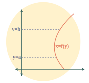 |
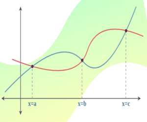
| Area between Two Curves | A = [Tex]\int_{a}^{b} [/Tex][f(x) – g(x)]dx
|  |
| Area between Compound Curves | A = [Tex]\int_{a}^{b} [/Tex][f(x) – g(x)]dx + [Tex]\int_{c}^{b} [/Tex][g(x) – f(x)]dx
|  |
| Area between Polar Curves | A = 1/2[Tex]\int_{\alpha}^{\beta} [/Tex]{(r0)2 – (ri)2}dθ |  |
Learn More, Area as Definite Integral
Volumes of Revolution
Volume of Revolution can be calculated using the formulas:
V = ∫ A(x) dx and V = ∫ A(y) dy
Where A(x) and A(y) represent the cross-sectional area functions with respect to the respective axis of rotation.
Learn More about Volumes of Revolution.
Arc Length
Arc length refers to the length of a curve between two given points. In calculus, finding the arc length of a curve involves integrating the distance formula along the curve’s path.
Given a curve represented by a function y = f(x) on an interval [a, b], the arc length formula for the curve is:
[Tex]L = \int_{a}^{b} \sqrt{1 + \left(\frac{dy}{dx}\right)^2} dx[/Tex]
Similarly, if the curve is represented parametrically by x = g(t) and y = h(t) on an interval [t1, t|2], the arc length formula becomes:
[Tex]L = \int_{t_1}^{t_2} \sqrt{\left(\frac{dx}{dt}\right)^2 + \left(\frac{dy}{dt}\right)^2} dt [/Tex]
Read More about Arc Length.
Improper Integral
An improper integral is an integral with one or both limits of integration being infinite or where the integrand function is unbounded within the interval of integration.
There are two types of improper integrals:
Type 1: The integrand becomes unbounded at one or both of the limits of integration. For example:
- [Tex]\int_{a}^{\infty} f(x) \, dx [/Tex]
- [Tex] \int_{-\infty}^{b} f(x) \, dx [/Tex]
- [Tex] \int_{-\infty}^{\infty} f(x) \, dx [/Tex]
To evaluate a Type 1 improper integral, you take the limit as a variable approaches infinity or negative infinity, depending on the case.
Type 2: The integrand becomes unbounded at a finite point within the interval of integration. For example:
- [Tex]\int_{a}^{b} \frac{f(x)}{(x – c)^p} ~ dx [/Tex]
Where p > 0 and a ≤ c ≤ b . Here, c is the point where the integrand becomes unbounded.
To evaluate a Type 2 improper integral, you split it into two integrals at the point of discontinuity c and then take limits for each integral.
Read More about Improper Integral.
Share your thoughts in the comments
Please Login to comment...