Integral Calculus

Integral Calculus is the branch of calculus that deals with topics related to integration. Integrals are major components of calculus and are very useful in solving various problems based on real life. Some of such problems are the Basel problem, the problem of squaring the circle, the Gaussian integral, etc. Integral Calculus is directly related to differential calculus.

This article is a brief introduction to Integral Calculus, including topics such as fundamental theorems of integral calculus, types of integral, and integral calculus formulas, definite and indefinite integrals with their properties, applications of integral calculus, and their examples.

What is Integral Calculus?

The process of finding the function from its derivative is called anti-derivative which is also referred to as Integration. In this process, the result obtained after the integration is called the integral. This integral and integration hold many properties and the study of these properties in the branch of mathematics is called Integral Calculus. Various methods in Integral Calculus are used in many ways such as to find the areas and volumes, approximate solutions of equations, calculate complex interactions of physical objects in our surroundings, etc.

Integral Calculus Definition

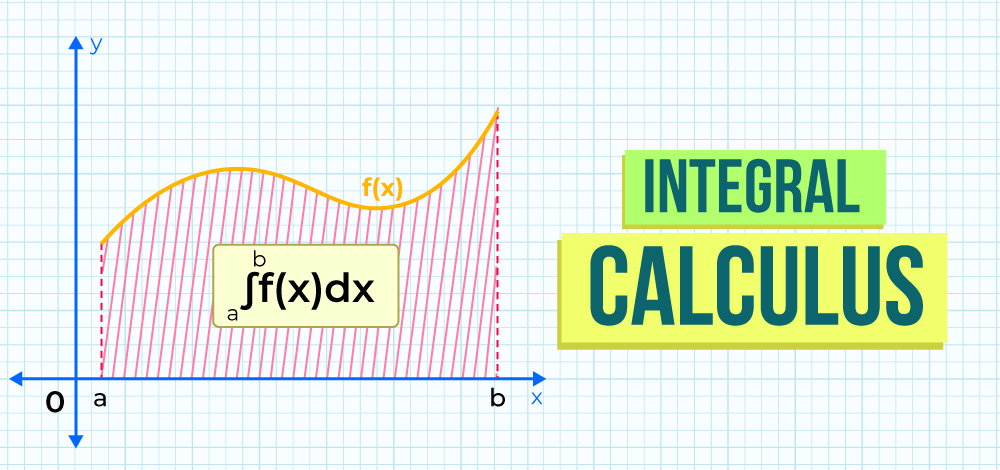
Integral calculus is a branch of mathematics focused on the concepts of integration. It involves finding the integral of a function, which represents the accumulation of quantities and can be interpreted as the area under a curve defined by the function over a specific interval

Fundamental Theorems of Integral Calculus

The integral represents the area under the curve. There are two fundamental theorems of integral calculus:

• First Fundamental Theorem of Integral Calculus
• Second Fundamental Theorem of Integral Calculus

First Fundamental Theorem of Integral Calculus

The first fundamental theorem of integral calculus states that if P(x) = ∫ f(x) dx is a continuous function on the interval [a, b], then P'(x) = f(x) for all x ∈ [a, b].

Second Fundamental Theorem of Integral Calculus

The second fundamental theorem of integral calculus states that if f(x) is a continuous function on the interval [a, b] and p(x) is the antiderivative of f(x), then [Tex]\int\limits_a^b  [/Tex]f(x) dx = p(b) – p(a) where the integral is called as a definite integral and a and b are called as lower and upper limits of the integral respectively.

Integral Definition

The antiderivative of the function f is called the integral of f. The reverse of differentiation is called as integration. The integral is also called as the primitive function of f or Newton-Leibnitz integral. The integral is the area under the curve. There are two types of integral: Definite integral and indefinite integral.

Types of Integrals

Integrals can be classified as:

• Definite Integral
• Indefinite Integral
• Improper Integrals

Definite Integrals

The definite integrals are the integrals which are bounded by the limits. The antiderivative p(x) of a continuous function f(x) on the interval [a, b] is called a definite integral. It is denoted by [Tex]\int\limits^b_a  [/Tex]f(x)dx and its value equals to p(b) – p(a) where p(b) is the antiderivative at x = b and p(a) is the antiderivative at x = a. The interval [a, b] is called interval of integration. The a and b are called the limits of integration where a is called the lower limit and b is called the upper limit of the integration. The definite integral does not require any constant integration.

Definite Integral Formula

To calculate the definite integral of any function, we can use the Second Fundamental Theorem of Integral Calculus, which is already discussed above. According to that, the formula for Definite Integral is:

[Tex]\bold{\int\limits^b_a}  [/Tex]f(x)dx = p(b) – p(a)

Where,

• p(b) is antiderivative of f(x) at x = b, and
• p(a) is antiderivative of f(x) at x = a.

Properties of Definite Integrals

Some properties of definite integrals are:

• [Tex]\int\limits^b_a  [/Tex]f(x) dx = [Tex]\int\limits^b_a  [/Tex]f(z) dz
• [Tex]\int\limits^b_a  [/Tex]f(x) dx = – [Tex]\int\limits^a_b  [/Tex]f(x) dx
• [Tex]\int\limits^b_a  [/Tex]f(x) dx = [Tex]\int\limits^c_a  [/Tex]f(x) dx + [Tex]\int\limits^b_c  [/Tex]f(x) dx
• [Tex]\int\limits^a_0  [/Tex]f(x) dx = [Tex]\int\limits^a_0  [/Tex]f(a – x) dx
• [Tex]\int\limits^a_{-a}f(x) dx = \begin{cases}2\int\limits_{0}^{a}f(x)dx&\text{, if $n$ is even}\\ 0&\text{, if $n$ is odd} \end{cases}  [/Tex]
• If f(x) is continuous function defined on [0, 2a] [Tex]\int\limits^{2a}_{0}f(x) dx = \begin{cases}2\int\limits_{0}^{a}f(x)dx&\text{, if f(2a – x) = f(x)}\\ 0&\text{,if f(2a – x) = – f(x) } \end{cases} [/Tex]
• [Tex]\int\limits^b_a  [/Tex]f(x) dx = [Tex]\int\limits^b_a  [/Tex]f(a + b – x) dx

Read More: Definite Integrals

Indefinite Integrals

The integrals that do not have the limit of integration are called indefinite integrals. The indefinite integrals involve the addition of constant of integration. The integration of the function f(x) is represented by F(x) and is given by

∫ f(x) dx = F(x) + C

Where,

• x is called the variable of integration,
• f(x) is called the integrand,
• F(x) is called as antiderivative of f(x), and
• C is called the constant of integration.

Read More: Indefinite Integral

Properties of Indefinite Integrals

There are several properties of integral calculus:

1. (d/dx)(∫ f(x) dx) = f(x)
2. ∫[k .f(x)] dx = k (x) dx, where k is constant
3. ∫{f(x) ± g(x)} dx = ∫ f(x) dx ± ∫g(x) dx

Improper Integrals

The integrals whose integrand is not bounded, or the limit of the integral is infinity, then the integral is called as improper integrals. Some examples of improper integrals are: [Tex]\int\limits_1^\infty  [/Tex]f(x)dx or [Tex]\int\limits^1_0  [/Tex][dx/x]

Multiple Integrals

Multiple integrals are integrals with more than one variable. There are two types of multiple integrals. They are:

• Double Integral
• Triple Integral

Double Integral

The integral of two variable functions under a specified region is called double integration. It is denoted by ∬.

Let’s see the following example to learn more about the process of double integral.

Example: Evaluate the double integral ∬_R x² + y² dA, where R is the region bounded by the curves y = x² and y = 2x.

Answer:

The curves y = x² and y = 2x intersect at the point (0, 0) and (2, 4).

Thus, the limit of integration for variable x is: 0 ≤ x ≤ 2.

and for interval [0, 2], x² ≤ 2x.

∬_R x² + y² dA = [Tex]\int_{0}^{2} \int_{x^2}^{2x} (x^2 + y^2) dy dx [/Tex]

Let I’ = [Tex]I’ = \int_{x^2}^{2x} (x^2 + y^2) dy [/Tex]

[Tex]\Rightarrow I’ = \int_{x^2}^{2x} (x^2 + y^2) \, dy \\ \Rightarrow I’ = \left[ x^2y + \frac{y^3}{3} \right]_{x^2}^{2x} \\ \Rightarrow I’ = 2x^3 + \frac{8x^3}{3} – \frac{x^6}{3} + \frac{x^6}{3} \\ \Rightarrow I’ = \frac{14x^3}{3} [/Tex]

Thus, ∬_R x² + y² dA = [Tex]\int_{0}^{2} \frac{14x^3}{3} dx [/Tex]

⇒ ∬_R x² + y² dA = [Tex]\frac{14}{3} \times \left[\frac{x^4}{4}\right]_{0}^{2} [/Tex]

⇒ ∬_R x² + y² dA = (14/3) × [(16/4) – 0]

⇒ ∬_R x² + y² dA = 56/3

Read More: Double Integral

Triple Integral

The integral of three variable functions under the 3-D region is called triple integration. It is denoted by ∭.

Let’s consider an example to learn how to calculate the triple integral.

Certainly! Here’s the direct solution using LaTeX code for the triple integral example:

Example: Evaluate the triple integral ∭_V xyz dV, where V is defined by 0 ≤ x ≤ 1, 0 ≤ y ≤ 2, and 0 ≤ z ≤ 3.

Solution:

Given the region V: 0 ≤ x ≤ 1, 0 ≤ y ≤ 2, and 0 ≤ z ≤ 3, the triple integral can be evaluated as follows:

[Tex]\begin{aligned} \iiint V xyz \, dV &= \int_{0}^{1} \int_{0}^{2} \int_{0}^{3} xyz \, dz \, dy \, dx \\ \Rightarrow \iiint V xyz &= \int_{0}^{1} \int_{0}^{2} \left[ \frac{xy z^2}{2} \right]_{0}^{3} \, dy \, dx \\ \Rightarrow \iiint V xyz &= \int_{0}^{1} \int_{0}^{2} \frac{27xy}{2} \, dy \, dx \\ \Rightarrow \iiint V xyz &= \int_{0}^{1} \left[ \frac{27xy^2}{4} \right]_{0}^{2} \, dx \\ \Rightarrow \iiint V xyz &= \int_{0}^{1} 27x \, dx \\ \Rightarrow \iiint V xyz &= \left[ \frac{27x^2}{2} \right]_{0}^{1} \\ \Rightarrow \iiint V xyz &= \frac{27}{2} \end{aligned} [/Tex]

So, the value of the triple integral ∭_V xyz dV over the region V is 27/2.

Integral Calculus Formulas

Integral calculus formulas are as follows:

• d/dx {(ϕ(x))} = f(x) ⇔ ∫ f(x) dx = ϕ(x) + C
• ∫xⁿ dx = (xⁿ⁺¹) / (n+1) + C, n ≠ 1
• ∫(1/x) dx = log_e|x| + C
• ∫ e^x dx = e^x + C
• ∫ a^x dx = (a^x / log_ea) + C
• ∫ sin x dx = – cos x + C
• ∫ cos x dx = sin x + C
• ∫sec²x dx = tan x + C
• ∫ cosec²x dx = -cot x + C
• ∫sec x tan x dx = sec x + C
• ∫ cosec x cot x dx = – cosec x + C
• ∫ cot x dx = log |sin x| + C
• ∫tan x dx = – log |cos x| + C
• ∫sec x dx = log |sec x + tan x| + C
• ∫ cosec x dx = log |cosec x – cot x| + C
• ∫ [1 /√(a² – x²)] dx = sin^-1(x/a) + C
• ∫ -[1 /√(a² – x²)] dx = cos^-1(x/a) + C
• ∫ [1 / (a² + x²)] dx = (1/a) tan^-1(x/a) + C
• ∫ -[1 / (a² + x²)] dx = (1/a) cot^-1(x/a) + C
• ∫ [1 / {x√(x² – a²)}] dx = (1/a) sec^-1(x/a) + C
• ∫ -[1 / {x√(x² – a²)}] dx = (1/a) cosec^-1(x/a) + C

Let’s consider some examples for better understanding.

Example 1: Solve: ∫x⁵dx

Solution:

∫x⁵dx = [x^{5 + 1} / (5 + 1)] + C

Using ∫xⁿ dx = (xⁿ⁺¹) / (n+1) + C, we get

∫x⁵dx = (x⁶ / 6) + C

Example 2: Find the definite integral of the function f(x) = 3x² + 2x – 5.

Answer:

Using ∫xⁿ dx = (xⁿ⁺¹) / (n+1) + C and ∫{f(x) ± g(x)} dx = ∫ f(x) dx ± ∫g(x) dx, we get

∫(3x² + 2x – 5) dx = 3x³/3 + 2x²/2 – 5x + C

Example 3: Evaluate the indefinite integral ∫(4e^x + 1/x) dx.

Answer:

As we know,

• ∫ e^x dx = e^x + C
• and ∫ kf(x) dx = k ∫ f(x) dx

∫ 4e^x dx = 4e^x + C₁

and ∫ 1/x dx = log x + C₂

⇒ ∫(4e^x + 1/x) dx = 4e^x + C₁ + log x + C₂

⇒ ∫(4e^x + 1/x) dx = 4e^x + log x + C₁ + C₂

⇒ ∫(4e^x + 1/x) dx = 4e^x + log x + + C [Where C = C₁ + C₂]

Methods to Find Integrals

There are multiple types of integrals which can be solved using different methods. Some integrals can be directly solved by applying formulas. To solve some integrals, we use the following methods:

• Integration by Substitution
• Integration by Parts
• Integration by Partial Fraction

Integration by Substitution

To understand the method of Integration by Substitution, we can see the following example or we can explore the article mentioned above.

Example: Evaluate: ∫[(2x)/ {5x² +1}]dx

Solution:

Let 5x² + 1 = t. Then, d(5x² + 1) = dt ⇒ 10 x dx = dt

⇒ ∫[(2x)/ {5x² +1}]dx = ∫[2x / (t×10x)]dt

⇒ ∫[(2x)/ {5x² +1}]dx = ∫[1 / (5t)]dt

⇒ ∫[(2x)/ {5x² +1}]dx = (1/5) ∫[1 / t]dt

⇒ ∫[(2x)/ {5x² +1}]dx = [(log t) / 5] + C

Integration by Parts

Let’s consider an example for better understanding.

Example: Evaluate the integral ∫e^x x dx

Solution:

Let I = ∫e^x x dx

This integral can be solved by integration by parts (ILATE rule)

According to ILATE rule the first function u = x (algebraic), v = e^x (exponent)

The formula of integration by parts

⇒ ∫u.v dx = u∫v dx – ∫[(du/dx)∫v dx] dx

⇒ ∫x e^x dx = x∫e^x dx – ∫[(dx/dx)∫e^x dx] dx

⇒ ∫x e^x dx = x e^x – ∫[(1)e^x] dx + C1

⇒ ∫x e^x dx = x e^x – ∫e^x dx + C1

⇒ ∫x e^x dx = x e^x – e^x + C1 + C2

⇒ ∫x e^x dx = e^x(x – 1) + C [C = C1 + C2]

Integration by Partial Fraction

For better understanding, let’s consider the following example.

Example: Evaluate the integral ∫[x/ {(x – 1)(x – 2)}]dx

Solution:

I = ∫[x/ {(x – 1)(x – 2)}]dx

These types of integrals can be solved using partial fraction method.

[x/ {(x – 1)(x – 2)}] = A/(x – 1) + B /(x – 2)

⇒ [x/ {(x – 1)(x – 2)}] = [A(x-2) + B(x-1)]/[(x – 1) (x – 2)]

Equating the numerators

x = A(x-2) + B(x – 1)

⇒ x = Ax + Bx -2A – B

⇒ x = (A + B)x – (2A + B)

Comparing coefficients

A + B = 1 . . . (1)

-2A – B = 0 . . . (2)

From (1) and (2)

B = -2A

Thus, A +(-2A) = 1

⇒ -A = 1

⇒ A = -1

Thus, B = 2

Putting values of A and B in (I)

[x/ {(x – 1)(x – 2)}] = (-1)/(x – 1) + 2 /(x – 2)

⇒ ∫[x/ {(x – 1)(x – 2)}] = ∫[(-1)/(x – 1) + 2 /(x – 2)] dx

⇒ ∫[x/ {(x – 1)(x – 2)}] = ∫[(-1)/(x – 1)]dx + ∫[2 /(x – 2)] dx

⇒ ∫[x/ {(x – 1)(x – 2)}] = -∫[1/(x – 1)]dx + 2∫[1 /(x – 2)] dx

⇒ ∫[x/ {(x – 1)(x – 2)}] = -ln(x – 1) + 2 ln(x – 2) + C1 + C2

⇒ ∫[x/ {(x – 1)(x – 2)}] = -ln(x – 1) + 2 ln(x – 2) + C [C=C1 + C2]

Applications of Integral Calculus

Integral calculus has different applications. Some of them are:

• To find the area under the curve.
• To find the area between two curves.
• To find the volumes.
• To find displacement and motion.

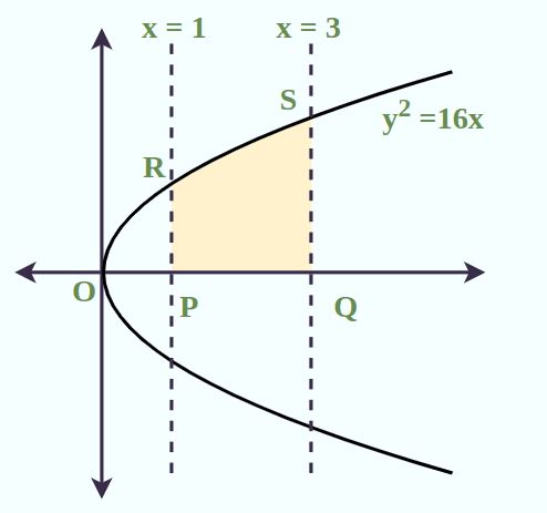
Example 1: Find the area of the region bounded by the curve y² = 16x, x = 1, x=3 and the x-axis in first quadrant.

Solution:

First, we draw the figure of the curve y² = 16x, x = 1, x=3 and the x-axis in first quadrant

y² = 16x

⇒ y = ±√(16x)

⇒ y = ±4√x . . . (1)

We will take positive value of y as we have to find area under the first quadrant.

The required area is the shaded region PQRS.

Required area = [Tex]\int\limits^3_1  [/Tex]y dx

⇒ Required area = \int\limits^3_1 4√xdx [From equation 1]

⇒ Required area = 4[x^½+1 / {(1/2)+1}]₁³

⇒ Required area = 4[x^3/2 / (3/2)]₁³

⇒ Required area = 4[(2x^3/2)/3]₁³

⇒ Required area = (8/3) [ 3^3/2 – 1^3/2]

⇒ Required area = (8/3) [3√3 – 1]

⇒ Required area = [8√3 – (8/3)] sq units

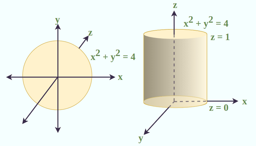
Example 2: Find the volume of solid bounded between the region x² +y² ≤ 4 and 0 ≤ z ≤ 1.

Solution:

From the given equation radius of disc = 2 units.

Required Volume = ∭_V dx dy dz

⇒ Required volume = ∬_R[Tex]\int\limits_{z=0}^{z=1} [/Tex](dz)dx dy

⇒ Required volume = ∬_R[z]₀¹dxdy = ∬_R[1 – 0]dx dy

⇒ Required volume = ∬_R[z]₀¹dxdy = ∬_R (1)dx dy

⇒ Required volume = ∬_R dx dy

Since, ∬_Rdx dy = Area (given shape is a disc which is a circle and area = πr² )

⇒ Required volume = π(2)²

⇒ Required volume = 4π cubic units

Example 3: Find the displacement of the particle over the interval [1, 3] if the velocity of the particle is given by v(t) = 3t² + 2t.

Solution:

Given the velocity v(t) = 3t² + 2t and the interval [1, 3]

Displacement S(t) = [Tex]\int\limits_a^b [/Tex]v(t) dt

Here, a = 1 and b = 3 by the given interval

⇒ S(t) = [Tex]\int\limits_1^3 [/Tex](3t² + 2t)dt

⇒ S(t) = [Tex]\int\limits_1^3 [/Tex]3t²dt + [Tex]\int\limits_1^3 [/Tex]2tdt

⇒ S(t) = 3[(t³/3)]₁³ + 2[(t²/ 2)]₁³

⇒ S(t) = [t³]₁³ + [t²]₁³

⇒ S(t) = [3³ – 1³] + [3² – 1²]

⇒ S(t) = [27 – 1] + [ 9 – 1]

⇒ S(t) = 26 + 8

⇒ S(t) = 34 units

The displacement is 34 units.

Differential vs Integral Calculus

The key differences between Differential calculus and Integral calculus are listed in the following table.

Differential Calculus	Integral Calculus
The differential calculus is the branch of mathematics that deals with derivatives.	The integral calculus is the branch of mathematics that deals with integrals.
The symbol of derivatives is d/dx.	The symbol of integral is ∫.
It gives the slope of the curve.	It gives the area under the curve.
The differentiation is opposite operation of integration.	The integration is opposite operation of differentiation.

People Also Read:

• Integrals | Definition, Meaning, Formula, Application
• Integration in Math: Definition, Formulas, Techniques
• Calculus in Maths
• List of Integral Formulas, Examples & FAQs

Integral Calculus Examples

Example 1: Solve: ∫x⁹dx

Answer:

∫x⁹dx = [x^{9 + 1} / (9 + 1)] + C

⇒ ∫x⁹dx = (x¹⁰ / 10) + C

Example 2: Solve ∫ 2^{x + 3}dx.

Answer:

∫ 2^{x + 3}dx = ∫ 2^x 2³dx

⇒ ∫ 2^{x + 3}dx = 8∫ 2^x dx

⇒ ∫ 2^{x + 3}dx = 8[2^x / log_e2] + C

Example 3: Evaluate: ∫(x³ + 3x² + 5x + 6)dx

Answer:

∫(x³ + 3x² + 5x + 6) dx = ∫x³dx + ∫ 3x²dx + ∫ 5x dx + ∫ 6dx

⇒ ∫(x³ + 3x² + 5x + 6) dx = (x³⁺¹ / (3+1)) + 3[(x²⁺¹ / (2+1))] + 5[(x¹⁺¹ / (1+1))] + 6[x⁰⁺¹/ (0+1)] + C

⇒ ∫(x³ + 3x² + 5x + 6) dx = (x⁴ / 4) + x³ + (5/2)x² + 6x + C

Example 4: Solve ∫(x + 6cos x) dx.

Answer:

∫(x + 6cos x) dx = ∫x dx + ∫cos x dx

⇒ ∫(x + 6cos x) dx = ∫x dx + 6 ∫cos x dx

⇒ ∫(x + 6cos x) dx = [x¹⁺¹ / (1+1)] + 6sin x + C

⇒ ∫(x + 6cos x) dx = [x² / 2] + 6sin x + C

Example 5: Evaluate ∫[1/{4√(x² – 16)}].

Answer:

∫[1/{4√(x² – 16)}] = ∫[1/{4√(x² – 4²)}]

⇒ ∫ [1 / {x√(x² – a²)}] dx = (1/a) sec^-1(x/a) + C

⇒ ∫[1/{4√(x² – 16)}] = (1/4) sec^-1(x/4) + C

Practice Problems on Integral Calculus

1. Calculate the integral of the function: ∫(3x² – 5x + 4) dx

2. Evaluate the integral involving a basic trigonometric function: ∫cos⁡(2x) dx

3. Use substitution to solve the integral: ∫x sin(x²) dx

4. Calculate the integral using the method of integration by parts: ∫x² e^x dx

5. Find the area under the curve from x = 0 to x = 𝜋 for the function: ∫₀^pi Sin(x) dx

FAQs on Integral calculus

What are Integrals?

The primitive value obtained after the integration is called the integral. The integrals are also called as antiderivative of the function.

What are the types of integrals?

There are two types of integrals:

• Definite Integrals
• Indefinite Integral

How to find the Integrals?

To evaluate we can use the integral calculus formulas, integration by substitution, integration by parts, integration by partial fraction.

Write some Applications of Integrals.

Some applications of integrals calculus are:

• To find the area of the curve
• To find the velocity from distance
• To find volumes of the solids
• To solve displacement and motion problems.

What is Definite Integral?

The antiderivative p(x) of the continuous function f(x) over the interval [a, b] is called definite integral. It is denoted by [Tex]\int\limits^b_a  [/Tex]f(x) dx and equals to p(b) – p(a) where p(b) and p(a) are antiderivatives at x= b and x =a respectively.

How Do You Use Integrals using Trigonometry?

Use the trigonometric identities and simplify the function into integrable function and then apply the formulas and adopt the integration procedures to find the integrals using trigonometry.