From revolutionizing computer vision to advancing natural language processing, the realm of artificial intelligence has ventured into countless domains. Yet, there’s one realm that’s been a consistent source of both fascination and complexity: audio. In the age of voice assistants, automatic speech recognition, and immersive audio experiences, the demand for robust, efficient, and scalable methods to process and understand audio data has never been higher. Enter the Audio Transformer, a groundbreaking architecture that bridges the gap between the visual and auditory worlds in the deep learning landscape.
Transformers
The transformer architecture has the ability to process all the parts of input in parallel through its self-attention mechanism without the need to sequentially process them.
The transformer architecture has two parts: an encoder and a decoder. The left side is the encoder, and the right side is the decoder. If we want to build an application to convert a sentence from one language to another (English to French), we need to use both the encoder and decoder blocks. This was the original problem (known as a sequence-to-sequence translation) for which the transformer architecture was developed. However, depending on the type of task, we can either use the encoder block only or the decoder block only of the transformer architecture.
.png)
Transformers
- For example, if we want to classify a sentence or a review as positive or negative, we need to use only the encoder part. The popular BERT is encoder-based, meaning it is built only using the encoder block of the transformer architecture.
- If we want to build an application for Question Answering, we can use the decoder block. The Chat GPT is a decoder-based model, meaning it is built using the decoder block of the transformer architecture.
The core of the encoder and decoder blocks is multi-head attention. The only difference is the use of masking in the decoder block. These layers tell the model to pay specific attention to certain elements in the input sequence and ignore others when computing the feature representations.
Using Transformers for Audio
To adapt the transformer architecture for audio applications, we can employ the conventional transformer structure outlined above, with a minor adjustment either in the input or output aspect to accommodate audio data instead of text. As these models fundamentally share the transformer architecture, their core architectural components remain similar, with the primary difference is the training methods and the processing of input or output data.
Audio Model Inputs
From the above discussion we can conclude that the input to audio model can either be text or audio.
Text Input
If the input is text then the original transformer architecture works as it is. The input text will be tokenized and passed through an embedding layer to get embedding vectors. This embedding vectors will be passed into the transformer encoder.
Audio Input
If the input is audio , we need to convert it to embedding vectors. In order to convert to embedding vectors we use 1d Convolution called as CNN feature encoder.
There are two approaches as to how we can pass the audio input through the CNN encoder:
- Feeding the raw audio (waveform audio) input directly into CNN feature encoder.
- Converting the raw audio into Log Mel Spectrogram or MFCC and then feeding into CNN feature encoder.
Waveform Audio Input
A waveform is a representation of an audio signal or any other continuous signal as a sequence of discrete data points. It’s a one-dimensional sequence of floating-point numbers. Each number in the sequence corresponds to the sampled amplitude of the signal at a particular point in time. These amplitudes are typically measured in terms of voltage or pressure variations in the analog signal. When we speak we cause disturbance in the air causing compression/decompression. This disturbance travels through the air and is called as sound wave. While speaking we generate sound waves with different frequencies simultaneously whose range is between 20 hz to 20000hz . Microphones capture this changes in air pressure and convert it into electrical energy. This electrical energy or signal is continuous and in order to store it we need to convert it to digital signal. This conversion is achieved through sampling that is we take the value of the signal at fixed interval of time and store it. If the sampling rate is 16khz it means in a 1 sec video with 16 khz sampling rate we store 16000 sample value .

Sound Wave Sampling
The above raw input is passed through a feature encoder. A typical feature encoder which was introduced in Wav2Vec2 model and is commonly used contains seven blocks and the temporal convolutions in each block have 512 channels with strides (5,2,2,2,2,2,2) and kernel widths (10,3,3,3,3,2,2). This results in an encoder output frequency of 49 hz with a stride of about 20ms between each sample, and a receptive field of 400 input samples or 25ms of audio. Detail calculation is shown below:
|
1 x 16000
|
10
|
5
|
512*3199
|
|
512 x 3199
|
3
|
2
|
512*1599
|
|
512 x 799
|
3
|
2
|
512*799
|
|
512 x 799
|
3
|
2
|
512*399
|
|
512 x 399
|
3
|
2
|
512*199
|
|
512 x 199
|
2
|
2
|
512*99
|
|
512 x 99
|
2
|
2
|
512*49
|
|
|
|
|

A typical process of feeding a raw audio input to Transformer Encoder
Spectrogram Inputs
A drawback associated with utilizing the raw waveform as input is its long sequence lengths. To illustrate, consider thirty seconds of audio recorded at a 16 kHz sampling rate, resulting in an input length of 30 * 16000 = 480,000. Longer sequence lengths results in increased computational demands within the transformer model, leading to high memory usage. Because of this, raw audio waveforms are not usually the most efficient form of representing an audio input. By using a spectrogram, we get the same amount of information but in a more compressed form. Two popular ways are to convert the raw input into MEL Spectrogram or MFCC. Lets discuss both :
- Mel Spectrogram
- In the real world in the most audio signals the frequency content varies over time. This is where the spectrogram comes in picture. We take a sound signal and divide the signal in small windows. We then compute Fourier transform of this windows. We plot the spectrum obtained for all the windows together which is know as spectrogram.
- The human ear has limitations in distinguishing closely spaced frequencies. This limitation becomes more noticeable as the frequencies get higher. For instance, we can easily tell the difference between a 500Hz and a 1000Hz frequency, but we struggle to differentiate between a 15000Hz and a 15500Hz frequency, even though the numerical difference is the same. In 1937, Stevens, Volkmann, and Newmann introduced the concept of the Mel scale, which provides a unit of pitch where equal pitch intervals sound equally spaced to a listener. To convert frequencies to the mel scale, we apply a specific mathematical operation.
- We aso don’t hear loudness on a linear scale. Generally to double the perceived volume of a sound we need to put 8 times as much energy into it. Therefore we take log of the amplitude. This is the decibel scale (The amplitude of a sound indicates the sound pressure level at a specific time and is measured in decibels (dB).).
- A Log-Mel spectrogram is a spectrogram where the frequencies are converted to the Mel scale and amplitude into decibels.
- Typically, in audio processing we divide the audio into 30-second segments, and for each segment, the Mel Spectrogram takes on a shape of (80, 3000), with 80 representing the number of Mel bins and 3000 as the sequence length. Through the transformation into a log-mel spectrogram, we not only decrease the volume of input data but also notably shorten the sequence length compared to the raw waveform. This log-mel spectrogram is subsequently passed through a feature enoder CNN as shown previously, resulting in a sequence of embeddings that can be fed into the transformer in the usual manner.
- Mel-frequency Cepstral Coefficients (MFCC)
- Another popular way of representing raw audio is to convert it to Mel-frequency cepstral coefficients (MFCC). MFCC is a very compressible representation, often using just 20 or 13 coefficients, they are a set of coefficients that capture the spectral characteristics of an audio signal.
- MFCCs are computed as follows
- Frame the signal into short frames: We frame the signal into 20 -40 ms (milli seconds) frames generally to get a reliable spectral estimate. Generally 25 ms is standard and a hop length of 10 ms is used. It means every 10 ms we will take 25 ms of audio. This allows overlap.
- A 16khz signal will be divided into 160 samples (16000 samples for 1 sec; 160 samples for 10 ms) each containing 400 frames (16000*.25)
- We compute the Discrete Fourier Transform (DFT) of each frame. This involves taking the absolute value of the complex Fourier transform and squaring the result, resulting in what is known as the Periodogram estimate of the power spectrum. Typically, a 512-point FFT is performed, retaining only the first 257 coefficients.
- Calculate a Mel-spaced filterbank – This comprises 20 to 40 triangular filters (with 26 being the common choice) applied to the power spectral estimate derived in step 2. Each filterbank is represented as a vector of length 257 (assuming the FFT settings from step 2). Most of the vector’s values are zeros, but a specific section corresponds to non-zero values. To compute filterbank energies, we multiply each filterbank by the power spectrum and sum the coefficients, yielding 26 values that represent the energy distribution across the filterbanks. Take the natural logarithm (log) of each of the 26 energies obtained in step 3, resulting in 26 log filterbank energies.
- We apply the Discrete Cosine Transform (DCT) to the 26 log filterbank energies, yielding 26 cepstral coefficients.
- For speech-related tasks, it’s common to retain only the lower 12 to 13 coefficients out of the 26.
- The resulting feature set, consisting of 12 numbers for each frame, is referred to as Mel Frequency Cepstral Coefficients (MFCCs)
We can pass Mel spectrogram or MFCC to a CNN Feature encoder which computes the embedding vector that is then consumed by transformer encoder. The 1d convolution is done along the time or sequence length. The Mel bins(80) or MFCC coefficients are taken as input channel for the 1d convolution
In both scenarios, whether dealing with waveform or spectrogram inputs, a common approach involves employing a compact neural network prior to utilizing the Transformer architecture. This initial network is responsible for transforming the input data into embeddings, after which the Transformer takes over to perform its specific task. This process ensures that relevant information is efficiently extracted from the input data before the Transformer works its magic.
Audio Transformer Outputs
The transformer architecture outputs a sequence of hidden-state vectors, also known as the output embeddings. Our goal is to transform these vectors into a text or audio output.
Text output
The objective of an automatic speech recognition model is to predict a sequence of textual tokens. To accomplish this, a language modeling head, typically comprising a single linear layer, is incorporated onto the transformer’s output. Subsequently, a softmax operation is applied to this head, enabling the prediction of probabilities for the various textual tokens within the vocabulary.
Spectrogram output
For models tasked with generating audio, such as a text-to-speech (TTS) model, additional layers must be incorporated to facilitate audio sequence generation. A common approach involves generating a spectrogram initially and subsequently utilizing an additional neural network, referred to as a vocoder, to transform this spectrogram into a waveform.
The output from the transformer network consists of a sequence of element vectors each of dimension d ( typically 768 ). A linear layer is employed to project this sequence into a log-Mel spectrogram. Following this, a post-net, composed of supplementary linear and convolutional layers, refines the spectrogram by mitigating noise. Finally, the vocoder takes this refined information to generate the ultimate audio waveform.

Generating Output through Decoder
Type Of Audio Architectures
Audio architectures can be broadly classified into two types :
Connectionist Temporal Classification (CTC)
These are encoder-only models that can be uses for either Automatic Speech Recognizations (ASR) or Audio classification task. These take the input features of audio, transform the input into a hidden state, and use a CTC head on top to predict the text.
Encoders are simpler models as compared to Seq2Seq but one downside is that they tend to predict the character for each input feature thereby requiring that the input and output have the same length which will not be true for our Automatic Speech Recognizations (ASR) tasks. This is where CTC helps in the realignment of input and output by allowing the model to predict the same character multiple times. Wav2Vec2 and M-CTC-T are examples of such architecture.
Let us see how an input is processed through a M-CTC-Large model. The M-CTC-T is a multilingual model i.e. a single model can transcribe the audio in all the 60 languages it was trained. It is a 1 Billion parameter model. It transcribes speech audio recordings into text. The input is audio and the output is the text. The architecture diagram from original paper is shown below.
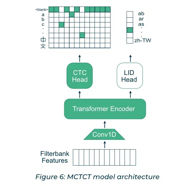
M-CTC-T model architecture
The main components of the M-CTC-T-Large model along with their dimensions are :
- Input – The input to the encoder is a sequence of 80-dimensional log Mel filterbank frames, extracted using 25 ms Hamming windows every 10ms from the 16 kHz audio signal. The maximum sequence length is 920
- Conv 1D – There is a single gated convolution layer (CONV1d + GLU)which performs convolution along the time axis(1D). This takes 80 input features of the log mel spectrum and convert it to a 3072 output feature. The filter length is 7 and it has a stride of 3 with valid padding. The GLU halves the output features to 1536.
- Encoder- These consist of 36 layers of below :
- Self-Attention: 4 heads of self-attention each of size 384. Thus the four attention combined take an input of 4*384 =1536 which is the output size of the convolution layer after GLU.
- Intermediate Layer : The encoder output is feed to intermediate layer which is a linear layer that transforms the feature vector from 1536 to 6144.
- Feed-forward Layer: The feedforward layer takes an input of 6144 and transforms it back to 1536. The final output of the encoder block is Batch * SeqLen * 1536
- CTC Head – The CTC head is a linear layer with 8065 outputs. One for each character of all the 60 languages. including punctuation, space, and the CTC blank symbol.
- LID (Language Identification) Head – The Lid head is a linear layer with 60 outputs – one for each language followed by mean pooling to aggregate along the sequence length. These LID outputs are used only during training.
Sequence to Sequence models (Seq2Seq)
These are encoder and decoder models allowing for different lengths of inputs and outputs as the input is processed by the encoder and the output is processed by the decoder. However, this model are complex and slower as compared to the CTC model. These are typically used for Automatic Speech Recognizations (ASR), Speech to Speech Translation and Speech Synthesis. Let us see how input is processed through a Seq2Seq model. We will take the example of Translatotron 2 architecture.
Translatotron is a speech-to-speech translation system translates the input audio from one language to another. The architecture includes:
- Input: The input to the encoder is the Mel-Spectrogram of the source speech. It takes 80 Mel channels. The frame size is of 25 ms and the frame step is 10 ms. The input is of size (batch, time, dim)
- The Encoder consists of below layers:
- Convolutional Subsampling Layer: Audio signal is initially passed through two layers of 2d Convolution with kernel size of 3, stride of 2, and output channel of 512. This effectively down samples the Mel-spectrogram to 1/4 or to a frame step of 40 ms. The output is of size (batch, sub-sampled time, sub-sampled dimension, output channel)
- Linear Layer: The output of the previous step is transformed to (batch, sub-sampled time, sub-sampled dimension*outputchanenel) and then passed through a linear layer to project the dimension to encoder dimension. The output of this layer is (batch, sub-sampled time, encoder_dim). The typical encoder dimension is of 512.
- Conformer Block: Its a combination of CNN + Transformer Encoder. A conformer block is composed of four modules stacked together, i.e., a feed-forward module, a self-attention module, a convolution module, and a second feed-forward module in the end.
- Feed-Forward Module: A feedforward module is composed of a normalization layer, two linear layers, one activation function(between the two linear layers), and a dropout. The first layer expands the dimension by an expansion factor and the second layer projects the expanded dimension back to the encoder dimension.
- Convolution Module: It consists of pointwisecon1d convolution which expands the channel by an expansion factor of 2 followed by GLU activation which halves the dimension back. This is followed by a depthwise 1D convolution with kernel size of 32 and a padding to keep dimensions the same followed by swish activation and a pointwise 1D convolution with the same number of channels in input and output. The final dimension of this block is (batch, sub-sampled time, encoder_dim)
- Multi-Head Self Attention : The number of attention heads is 4 and the number of layers is 17. The encoding dimension is divided among the attention head. Thus the output of the attention layer is (batch, sub-sampled time, encoder_dim)
- Feed-Forward Module: The same feedforwad module as above is repeated. The output dimesnion is (batch, sub-sampled time, encoder_dim)

Conformer Encoder Model
- Attention Module: The attention module serves as the bridge that connects all elements of the Translatotron architecture, including the encoder, decoder, and synthesizer. Number of attention head is 8 . The hidden dimension is 512 divided among the attention head. Thus the output dimension of the attention head is the same as that of the input – (batch,sub-sampled time, encoder_dim).
- Decoder: The autoregressive decoder is responsible for producing linguistic information in the translation speech. It takes the attention module, and predicts a phoneme sequence corresponding to the translation speech. It uses LSTM stack . The dimension of LSTM is same as encoder_dim. The number of stack is 6 to 4.The output from the LSTM stack is passed through a projection layer to convert it to phoneme embedding dimension which is typically 256
- Speech Synthesizer: It accepts two inputs: the intermediate output from the decoder (prior to the final projection and softmax for phoneme prediction) and the contextual output derived from the attention mechanism. These inputs are concatenated, and the synthesizer utilizes this combined information to produce a mel-spectrogram that corresponds to the translated speech.
- Vocoder: The spectrogram is subsequently input into a Vocoder, an abbreviation for “Voice” and “Encoder” to generate speech audio. Vocoders work by analyzing the spectral envelope and fundamental frequency (pitch) of the source speech, and then applying this information to synthesize speech in the target language.

Translatotron 2 Architecture
Conclusions
In conclusion, this article has provided an in-depth overview of how the powerful Transformer architecture, initially designed for natural language processing, can be adapted and extended for audio applications. There are two main types of audio architectures discussed: Connectionist Temporal Classification (CTC) models and Sequence-to-Sequence (Seq2Seq) models, each suited for different tasks within the realm of audio processing.
We also discussed the different forms of audio input, either raw waveform audio or spectrogram representations (such as Mel Spectrograms or MFCCs), and how these inputs are processed through a feature encoder before being fed into the Transformer architecture.
The output of these models can be text, generated by language modeling heads for ASR, or audio, where additional components like vocoders are used to synthesize the audio waveform from Mel-Spectrograms. This process allows for a seamless transition from audio to text or vice versa.
Share your thoughts in the comments
Please Login to comment...