Understand Audio data

Our daily lives are full of various audio in the form of sounds and speeches. Analyzing them is now a crucial task for numerous industries like Music, Crime Investigation, speech recognition, etc. Audio data analysis involves the exploration and interpretation of sound signals by extracting valuable insights, recognizing patterns, and making informed decisions. This multifaceted field encompasses a variety of fundamental concepts and techniques, contributing to a deeper comprehension of audio data. In this article, we will see various techniques to understand audio data.

Audio data

Audio is the representation of sound as a set of electrical impulses or digital data. It is the process of converting sound into an electrical signal that may be stored, transferred, or processed. The electrical signal is subsequently transformed back into sound, which a listener may hear.

Audio is a way to communicate our lives, and it influences how we connect with one another and perceive the world around us.

For this implementation, we need an audio data file (.wav). Let’s understand audio data using ‘Recording.wav’, which can be directly downloaded from here. You can use any audio file (.wav) at your convenience.

Understanding audio data step-by-step

Importing libraries

At first, we will import all the required Python libraries, like Librosa, NumPy, Matplotlib and SciPy.

• Librosa is a Python package for analyzing music and audio. It offers the components required to build music information retrieval systems.
• Scipy is a library used for scientific computation that offers helpful functions for signal processing, statistics, and optimization.
• Soundfile is a library to read and write sound files.

Python3

import librosa
import numpy as np
import matplotlib.pyplot as plt
from scipy.fft import fft
from scipy.signal import spectrogram
import soundfile as sf

Sampling and sampling rate

To understand the audio data, first we need to understand the Sampling and sampling rate.

• Sampling: We can understand audio signal very effectively by sampling in which continuous analog audio signals converted into discrete digital values. It measures the amplitude of the audio signal at regular intervals in time.
• Sampling rate: This is the number of total samples taken per second during the analog-to-digital conversion process. The sampling rate is measured in hertz (Hz).

Since human voice has audible frequencies below 8 kHz, sampling speech at 16 kHz is adequate. A faster sample rate just raises the computing cost of processing these files.

In the code, we will use Librosa module to sample audio file implicitly. It will first read the audio file and then convert it into a waveform (a sequence of amplitude values) that can be processed digitally.

Python3

# Load the audio file
audio_file = 'Recording.wav'
# sr set to none to extract sampling rate information from the audio file's metadata
waveform, sampling_rate = librosa.load(audio_file, sr=None)
print(f'Sampling Rate: {sampling_rate} Hz')

Output:

Sampling Rate: 48000 Hz

The sampling rate for the audio used is 48000 Hz.

Listen the Audio files at same Sampling Rate:

Python3

from IPython.display import Audio

Audio(waveform, rate=sampling_rate)

Output:

Sampling Rate : 4800

Listen the Audio files at Double Sampling Rate:

Python3

Audio(waveform, rate=sampling_rate*2)

Output:

Sampling Rate:9600

Listen the Audio files at half Sampling Rate:

Python3

Audio(waveform, rate=sampling_rate/2)

Output:

Sampling Rate: 2400

we will observe from the above audio that while changing the sampling rate audio are distorted.

Calculating Amplitude and Bit depth

Amplitude and Bit depth are two important concepts to understand the intensity of Audio Signal.

• Amplitude: It is the intensity of an audio signal at a particular point of time which corresponds to the height of the waveform at that instant of time. The amplitude is measured in decibels (dB). Human perceive amplitude of the sound wave as loudness. A rock concert can be around 125 dB, which is louder than a regular speaking voice and outside the range of human hearing.
• Bit depth: How precisely this amplitude value can be defined depends on the bit depth of the sample. The digital representation more closely resembles the actual continuous sound wave the higher the bit depth. Higher bit depth results better audio quality. For common audio files Bit depths can be 8 bits, 16 bits or 24 bits. We will print the amplitude range by subtracting maximum amplitude and minimum amplitude levels.

In the code snippet, calculates the amplitude range of the waveform. The soundlife library to stores the audio file in variable audio_data.

The code line bit_depth = audio_data.dtype.itemsize calculates the bit depth of the audio data by examining the data type of the audio_data array and finding its item size in bytes.

Python3

# Compute the amplitude range
amplitude_range = np.max(waveform) - np.min(waveform)
# Get the bit depth from the audio data
audio_data, sampling_rate = sf.read(audio_file)
bit_depth = audio_data.dtype.itemsize
# printing values
print(f'Amplitude Range: {amplitude_range}')
print(f'Bit Depth: {bit_depth} bits')

Output:

Amplitude Range: 0.292144775390625
Bit Depth: 8 bits

So, our audio file is in 8 bits category of bit depth.

Knowing the amplitude range and bit depth helps us to gain useful insights into the characteristics of an audio file, which is important in audio processing and analysis tasks.

Waveform (Time Domain) Representation

A waveform is the graphical representation of of an audio signal in the time domain where each point on the waveform represents the amplitude of the audio signal at a specific point in time. It will help us to understand how the audio signal varies over time by its revealing features like sound duration, pauses and amplitude changes.

In the code snippet, we have plot waveform leveraging librosa and matplotlib.

Python3

# Plot the waveform
## set size
plt.figure(figsize=(8, 4))

## Display the waveform of the adio signal
librosa.display.waveshow(waveform, sr = sampling_rate)
plt.xlabel('Time')
plt.ylabel('Amplitude')
plt.title('Audio Waveform')
plt.grid(True)
plt.show()

Output:

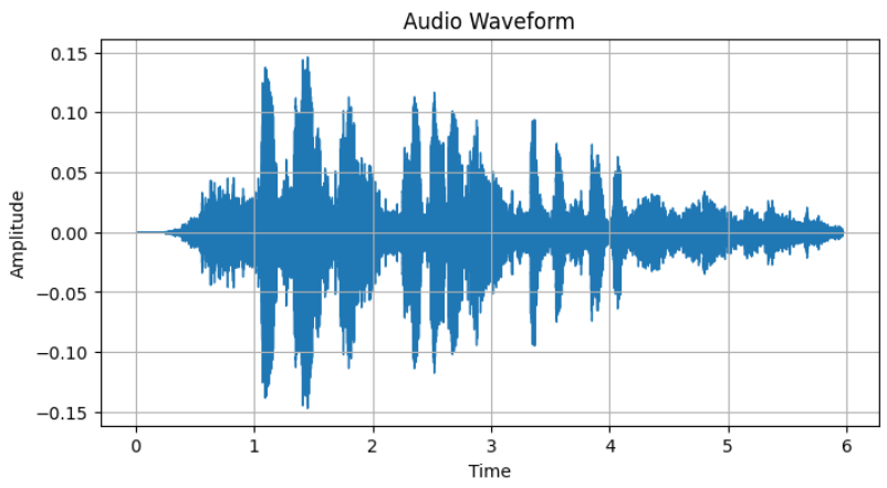
Waveform Representation

Visualizing Frequency Spectrum

Frequency Spectrum is a representation of how the energy in an audio signal is distributed across different frequencies which can be calculated by applying a mathematical transformation like the Fast Fourier Transform (FFT) to the audio signal. It is very useful for identifying musical notes, detecting harmonics or filtering specific frequency components.

The code snippet computes Fast Fourier Transform and plots frequency spectrum of audio using matplotlib.

Python3

# Compute the FFT of the waveform
spectrum = fft(waveform)

# Frequency bins
frequencies = np.fft.fftfreq(len(spectrum), 1 / sampling_rate)

# Plot the frequency spectrum
plt.figure(figsize=(8, 4))
plt.plot(frequencies[:len(frequencies)//2], np.abs(spectrum[:len(spectrum)//2]))
plt.xlabel('Frequency (Hz)')
plt.ylabel('Amplitude')
plt.title('Frequency Spectrum')
plt.grid(True)
plt.show()

Output:

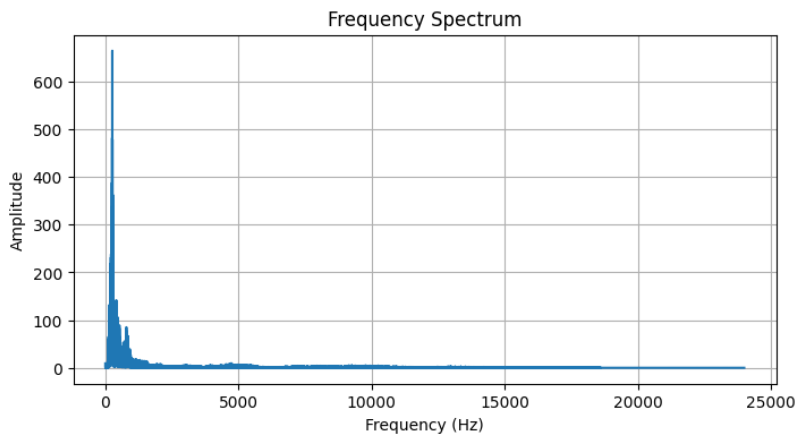
Frequency Spectrum

The plot displays the frequency of the audio signal, which allows us to observe the dominant frequencies and their amplitudes.

Spectrogram

Spectrogram is a time-frequency representation of an audio signal which provides a 2D visualization of how the frequency content of the audio signal changes over time.

In spectrogram, the dark regions indicate less presence of a frequency and in the other hand bright regions indicate strong presence of a frequency at a certain time. This will help is various tasks like speech recognition, musical analysis and identifying sound patterns.

The code snippet computes and plots the audio waveform using matplotlib library and scipy.signal.spectrogram function. In the code, epsilon defines a small constant to avoid division by zero. Epsilon is added to the spectrogram values before taking logarithm to prevent issues with very small values.

Python3

# Compute the spectrogram

# Small constant to avoid division by zero(if any)
epsilon = 1e-40
f, t, Sxx = spectrogram(waveform, fs=sampling_rate)

# Plot the spectrogram with the constant added to Sxx
plt.figure(figsize=(8, 4))
plt.pcolormesh(t, f, 10 * np.log10(Sxx + epsilon))
plt.colorbar(label='Power/Frequency (dB/Hz)')
plt.xlabel('Time (s)')
plt.ylabel('Frequency (Hz)')
plt.title('Spectrogram')
plt.show()

Output:

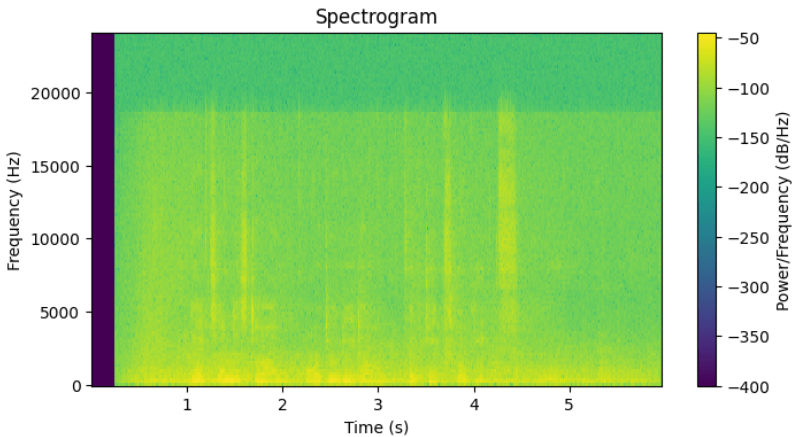
Spectrogram

The plot displays spectrogram, which represents how the frequencies in the audio signal change over time. The color intensity represents whether the frequency is high or low at each time point.

Conclusion

We can conclude that various types of visualization tasks help us to understand the behavior of audio signals very effectively. Also understanding audio signal is very essential task for audio classification, music genre classification and speed recognition.