Audio classification using spectrograms

Our everyday lives are full of various types of audio signals. Our brains are capable of distinguishing different audio signals from each other by default. But machines don’t have this capability. To learn audio classification, different approaches can be used. One of them is classification using spectrograms. Audio classification is an important task that is required for various applications like speech recognition, music genre classification, environmental sound analysis, forensic departments, and many more. In this article, we will explore the implementation guide for classifying audio signals using Spectrogram.

What is a spectrogram?

A spectrogram is a visual 2D representation of audio signals in the frequency domain that displays how the frequencies within a sound evolve over time by breaking down an audio signal into small segments and computing the intensity of different frequency components within each segment. The spectrogram, or time-frequency representation of an audio signal, helps us to understand valuable insights about the audio content, like distinguishing between various sounds, patterns, or characteristics. The efficient creation of spectrograms is a key step in audio classification using spectrograms. This spectrogram creation process involves various steps, which are discussed below.

1. Segmentation: At first, the raw audio signals are divided into short, overlapping time segments, or frames.
2. Frequency Analysis: segment, For each time segment, the Fourier transform is applied to obtain a frequency domain representation of that segment, which reveals the frequency components present in that short duration.
3. Repeat for Each Segment: This process is repeated for each time segment to create a series of individual frequency domain representations.
4. Mel spectrogram generation: In this article, we have used Mel spectrograms which is a representation of an audio signal that is closer to how humans perceive sound. This process starts with Fourier transformation and then a series of additional transformations are applied which models the nonlinear human auditory system’s response to different frequencies. It utilizes mel-scale which is a perceptual scale that emphasizes lower frequencies and de-emphasizes higher frequencies by mimicking how the human ear perceives sound. This is greatly useful for audio classification using Spectrograms.
5. Visualization: These frequency domain representations are then stacked horizontally which forms the spectrogram. Brightness or color intensity is used to represent the amplitude or energy of each frequency component in each frame.

The fourth step is an extra step which is only performed for audio classification. Please find the ‘Data pre-processing’ sub-section.

About the dataset

You can download the Barbie Vs Puppy dataset from here.

Step-by-step implementation

Importing required libraries

We will import all necessary Python libraries like NumPy, Sckit Learn, Matplotlib, Librosa etc.

Python3

import zipfile
import os
import librosa
import numpy as np
import matplotlib.pyplot as plt
from sklearn.model_selection import train_test_split
from sklearn.preprocessing import LabelEncoder
from sklearn.metrics import accuracy_score, f1_score
from sklearn.ensemble import GradientBoostingClassifier

Un-zipping the dataset

Our dataset is a zip file which contains audio files(.wav) in two respective folders. So, our first task is to extract its contains to out runtime.

Python3

# Path to the zip file containing the dataset
zip_file_path = "/content/archive.zip"

# Destination directory to extract the contents
extracted_dir = "/content/barbie_vs_puppy"

# Extract the contents of the zip file
with zipfile.ZipFile(zip_file_path, 'r') as zip_ref:
    zip_ref.extractall(extracted_dir)

Data pre-processing

It is the most important step when we are attempting to perform audio classification using spectrograms. We will load each of the audio files till 3s for spectrogram generation as per machine capabilities. You can extent it if required. In our present dataset most of the audio files are within a range of 3s. Here we will generate mel-Spectrograms for better classification.

Python3

# Set the path to dataset folder
data_dir = "/content/barbie_vs_puppy/barbie_vs_puppy"

# Load and preprocess audio data using spectrograms
labels = os.listdir(data_dir)
audio_data = []
target_labels = []

for label in labels:
    label_dir = os.path.join(data_dir, label)
    for audio_file in os.listdir(label_dir):
        audio_path = os.path.join(label_dir, audio_file)
        y, sr = librosa.load(audio_path, duration=3)  # Load audio and limit to 3 seconds
        spectrogram = librosa.feature.melspectrogram(y=y, sr=sr)
        spectrogram = librosa.power_to_db(spectrogram, ref=np.max)
        # Transpose the spectrogram to have the shape (timesteps, n_mels)
        spectrogram = spectrogram.T
        audio_data.append(spectrogram)
        target_labels.append(label)

Encoding targets and data-splitting

In this step, we will use Label Encoder to encode the target labels and then we will split the dataset into training and testing(80:20). After that we will scale all to spectrograms to a certain length to ensure all the spectrograms have same length. Otherwise, we can not be able to classify them.

Python3

# Encode target labels
label_encoder = LabelEncoder()
encoded_labels = label_encoder.fit_transform(target_labels)

# Split data into training and testing sets
X_train, X_test, y_train, y_test = train_test_split(audio_data, encoded_labels, test_size=0.2, random_state=42)

# Ensure all spectrograms have the same shape
max_length = max([spec.shape[0] for spec in audio_data])
X_train = [np.pad(spec, ((0, max_length - spec.shape[0]), (0, 0)), mode='constant') for spec in X_train]
X_test = [np.pad(spec, ((0, max_length - spec.shape[0]), (0, 0)), mode='constant') for spec in X_test]

# Convert to NumPy arrays
X_train = np.array(X_train)
X_test = np.array(X_test)

Exploratory data analysis

Now we will perform EDA to gain knowledge about dataset.

• Target class distribution: The distribution of the classes(here barbie and puppy) of target variable helps us to gain a deep knowledge and for assessing class balance and potential data biases.

Python3

# Count the number of samples in each class
class_counts = [len(os.listdir(os.path.join(data_dir, label))) for label in labels]
# Define colors for each class
class_colors = ['blue', 'green']
# Create a bar chart to visualize class distribution
plt.figure(figsize=(5, 3))
plt.bar(labels, class_counts, color=class_colors)
plt.xlabel("Class Labels")
plt.ylabel("Number of Samples")
plt.title("Class Distribution")
plt.show()

Output:

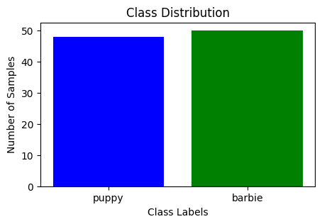
Distribution of classes

• Class-wise Spectrogram comparison: As we are performing audio classification using spectrogram so it is mandatory to visualize pattern of audio waveform and spectrograms for each class. Now both the target classes contains multiple number of audio files and we can visualize all of them if it is required. In this article, we will visualize only one spectrogram and waveform from each class.

Python3

# Define a function to plot spectrograms for a class
def plot_spectrograms(label, num_samples=3):
    label_dir = os.path.join(data_dir, label)
    plt.figure(figsize=(7, 4))
    plt.suptitle(f"Spectrogram Comparison for Class: {label}")

    for i, audio_file in enumerate(os.listdir(label_dir)[:num_samples]):
        audio_path = os.path.join(label_dir, audio_file)
        y, sr = librosa.load(audio_path, duration=3)
        spectrogram = librosa.feature.melspectrogram(y=y, sr=sr)
        spectrogram = librosa.power_to_db(spectrogram, ref=np.max)

        plt.subplot(num_samples, 2, i * 2 + 1)
        plt.title(f"Spectrogram {i + 1}")
        plt.imshow(spectrogram, cmap="viridis")
        plt.colorbar(format="%+2.0f dB")
        plt.xlabel("Time")
        plt.ylabel("Frequency")

        plt.subplot(num_samples, 2, i * 2 + 2)
        plt.title(f"Audio Waveform {i + 1}")
        plt.plot(np.linspace(0, len(y) / sr, len(y)), y)
        plt.xlabel("Time (s)")
        plt.ylabel("Amplitude")

    plt.tight_layout(rect=[0, 0, 1, 0.95])
    plt.show()


# Visualize spectrograms and audio waveforms for "barbie" class
# adjust num_samples parameter to see desired number of  visualization of samples
plot_spectrograms("barbie", num_samples=1)
print('\n')
# Visualize spectrograms and audio waveforms for "puppy" class
plot_spectrograms("puppy", num_samples=1)

Output:

Waveform and spectrogram comparison for ‘barbie’ class

Waveform and spectrogram comparison for ‘puppy’ class

Model fitting and evaluation

After EDA, we can say that we are going to perform Binary classification of audio as there are only two classes(barbie and puppy) present as target. So, we can choose a wide range of classification models for this task. Here, we are going to implement Gradient Boosting classifier of ensemble learning technique. We will pass all parameters of its to there default values. Only one parameter called ‘random_state‘ will be specified to handle the randomness during model training and to ensure that the model will produce same result for each execution. Finally, we will evaluate this model’s performance in the terms of accuracy and F1-score.

Python3

# Convert the data to a flat 2D shape
X_train_flat = X_train.reshape(X_train.shape[0], -1)
X_test_flat = X_test.reshape(X_test.shape[0], -1)

# Create Gradient Boosting classifier
model = GradientBoostingClassifier(random_state=42)
# Train the model
model.fit(X_train_flat, y_train)

# Make predictions
y_pred = model.predict(X_test_flat)

# Calculate accuracy and F1 score
accuracy = accuracy_score(y_test, y_pred)
f1 = f1_score(y_test, y_pred)

print("Accuracy: {:.4f}".format(accuracy))
print("F1 score: {:.4f}".format(f1))

Output:

Accuracy: 0.7500
F1 score: 0.8000

Note: By using same data-preprocessing code you can implement different classifier models as per your choice. Only for example Gradient Boosting classifier is implemented. All other model implementation will be same as it is.

Conclusion

We can conclude that, Audio classification using spectrogram is a long and calculative technique. However, it can effectively useful for audio classification. Our model performed moderately well with a accuracy of 65% and achived a decent F1-score of approximately 70%. These results show that audio classification using spectrogram may be a lengthy process but by using correct model and hyperparameter-tuning, we can achieve outstanding results for classification of audio.