Discrete Fourier Transform and its Inverse using MATLAB
Last Updated :
04 Jul, 2021
With the advent of MATLAB and all the scientific inbuilt that it has brought, there’s been a significant change and simplification of sophisticating engineering scenarios. In fact, this change has contributed to helping build better visualization and practical skills for students pursuing technical studies in the sciences, if not other fields at the very least. Here we look at implementing a fundamental mathematical idea – the Discrete Fourier Transform and its Inverse using MATLAB.
Calculating the DFT
The standard equations which define how the Discrete Fourier Transform and the Inverse convert a signal from the time domain to the frequency domain and vice versa are as follows:
DFT:  for k=0, 1, 2….., N-1
IDFT:  for n=0, 1, 2….., N-1
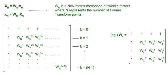
The equations being rather straightforward, one might simply execute repetitive/nested loops for the summation and be done with it. However, we should attempt to utilize another method where we use matrices to find the solution to the problem. Many readers would recall that the DFT and IDFT of a time/frequency domain signal may be represented in vector format as the following:


When we take the twiddle factors as components of a matrix, it becomes much easier to calculate the DFT and IDFT. Therefore, if our frequency-domain signal is a single-row matrix represented by XN and the time-domain signal is also a single-row matrix represented as xN……
With this interpretation, all we require to do, is create two arrays upon which we shall issue a matrix multiplication to obtain the output. The output matrix will ALWAYS be a Nx1 order matrix since we take a single-row matrix as our input signal (XN or xN). This is essentially a vector which we may transpose to a horizontal matrix for our convenience.
Algorithm (DFT)
- Obtain the input sequence and number of points of the DFT sequence.
- Send the obtained data to a function which calculates the DFT. It isn’t imperative to declare a new function but code legibility and flow become cleaner and apparent.
- Determine the length of the input sequence using the length( ) function and check if the length is greater than the number of points. N must always be equal to or greater than the sequence. If you try to execute the matrix multiplication by not satisfying the condition, you’ll be met with an error in your command window.
- Accounting for the difference in lengths of the input sequence and the N-points using a separate array which adds extra zeros to elongate the input sequence. This is done using the zeros(no_of_rows, no_of_columns) function which creates a 2D array composed of zeros.
- Based on the value of N obtained as input, create the WN matrix. To do this, implement 2 ‘for’ loops -quite a basic procedure.
- Simply multiply the two arrays that have been created. This is an array of the required frequency-domain signal samples.
- Plot the magnitude and the phase of the output signal via inbuilt functions abs(function_name) and angle(function_name).
Matlab
clc;
xn=input('Input sequence: ');
N = input('Enter the number of points: ');
Xk=calcdft(xn,N);
disp('DFT X(k): ');
disp(Xk);
mgXk = abs(Xk);
phaseXk = angle(Xk);
k=0:N-1;
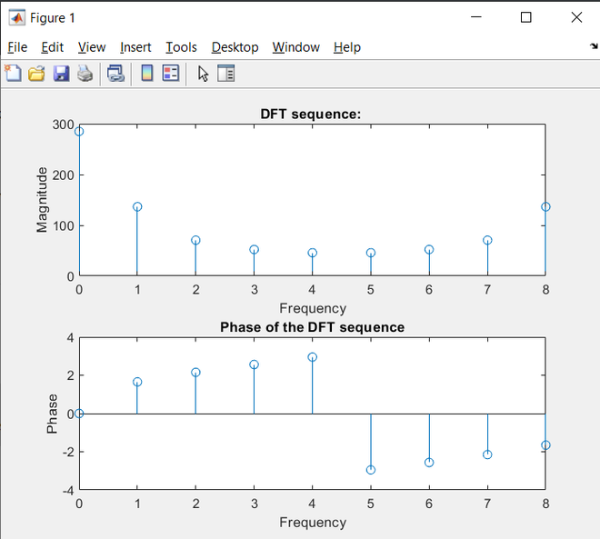
subplot (2,1,1);
stem(k,mgXk);
title ('DFT sequence: ');
xlabel('Frequency');
ylabel('Magnitude');
subplot(2,1,2);
stem(k,phaseXk);
title('Phase of the DFT sequence');
xlabel('Frequency');
ylabel('Phase');
function[Xk] = calcdft(xn,N)
L=length(xn);
if(N<L)
error('N must be greater than or equal to L!!')
end
x1=[xn, zeros(1,N-L)];
for k=0:1:N-1
for n=0:1:N-1
p=exp(-i*2*pi*n*k/N);
W(k+1,n+1)=p;
end
end
disp('Transformation matrix for DFT')
disp(W);
Xk=W*(x1.')
end
|
Output:
>> Input sequence: [1 4 9 16 25 36 49 64 81]
>> Enter the number of points: 9
Algorithm (IDFT)
- Obtain the frequency-domain signal / sequence as input (X(k)). The length of this sequence suffices as a value for N (points).
- Pass this array to a function for computation.
- Run 2 loops in the function to create the matrix. Note that this matrix must be conjugated when being utilized for the calculation. You may choose to explicitly declare another array which is the conjugate of the matrix WN.
- Once, the matrix has been created, obtain the conjugate using ‘*‘ and simply multiply it with the input sequence’s transpose. We require the transpose as the input is a row matrix. When multiplying with the WN matrix we have created, the number of columns in WN must match the number of rows in X(k).
- Plot this sequence using stem(x_axis, y_axis). DO NOT use plot( ) since this is not a CT signal.
Matlab
clc;
Xk = input('Input sequence X(k): ');
xn=calcidft(Xk);
N=length(xn);
disp('xn');
disp(xn);
n=0:N-1;
stem(n,xn);
xlabel('time');
ylabel('Amplitude');
function [xn] = calcidft(Xk)
N=length(Xk);
for k=0:1:N-1
for n=0:1:N-1
p=exp(i*2*pi*n*k/N);
IT(k+1,n+1)=p;
end
end
disp('Transformation Matrix for IDFT');
disp(IT);
xn = (IT*(Xk.'))/N;
end
|
Output:
>> Enter the input sequence: [1 2 3 4 5 9 8 7 6 5]
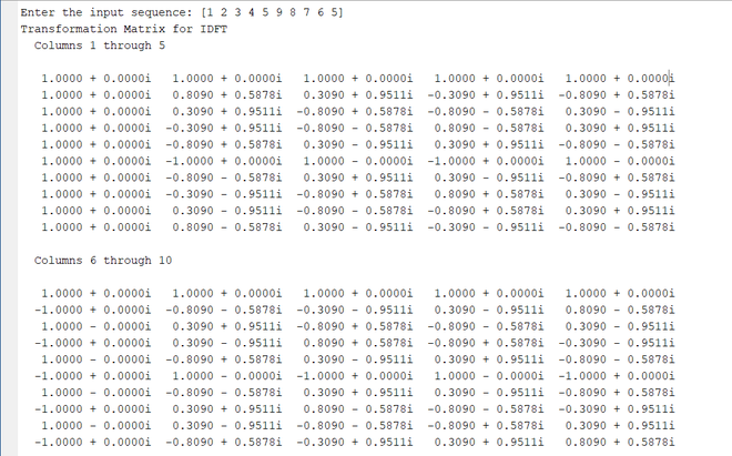
Transformation Matrix
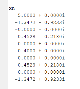
The time-domain sequence
Share your thoughts in the comments
Please Login to comment...