Statistics Cheat Sheet

Statistics is like a toolkit we use to understand and make sense of information. It helps us collect, organize, analyze, and interpret data to find patterns, trends, and relationships in the world around us.

In this Statistics cheat sheet, you will find simplified complex statistical concepts, with clear explanations, practical examples, and essential formulas. This cheat sheet will make things easy when getting ready for an interview or just starting with data science. It explains stuff like mean, median, and hypothesis testing with examples, so you’ll get it in no time. With this cheat sheet, you’ll feel more sure about your stats skills and do great in interviews and real-life data jobs!

What is Statistics?

Statistics is the branch of mathematics that deals with collecting, analyzing, interpreting, presenting, and organizing data. It involves the study of methods for gathering, summarizing, and interpreting data to make informed decisions and draw meaningful conclusions.

Statistics is widely used in various fields such as science, economics, social sciences, business, and engineering to provide insights, make predictions, and guide decision-making processes. Statistics is like a tool that helps us see patterns, trends, and relationships in the world around us. Whether it’s counting how many people like pizza or figuring out the average score on a test, statistics helps us make decisions based on data. It is used in lots of different areas, like science, business, and even sports, to help us learn more about the world and make better choices.

Types of Statistics

There are commonly two types of statistics, which are discussed below:

1. Descriptive Statistics: De­scriptive Statistics helps us simplify and organize big chunks of data. This makes large amounts of data easier to understand.
2. Inferential Statistics: Inferential Statistics is a little different. It uses smaller data to conclude a larger group. It helps us predict and draw conclusions about a population.

Basics of Statistics

Basic formulas of statistics are,

Parameters	Definition	Formulas
Population Mean, (μ)	Entire group for which information is required.	∑x/N
Sample Mean	Subset of population as entire population is too large to handle.	∑x/n
Sample/Population Standard Deviation	Standard Deviation is a measure that shows how much variation from the mean exists.	[Tex]\\\sqrt\frac{{\sum(x-\overline{x})^2}}{n-1}[/Tex]
Sample/Population Variane	Variance is the measure of spread of data along its central values.	[Tex]Variance(Population)~=~\frac{{\sum(x-\overline{x})^2}}{n}\\ Variance(Sample)~=~\frac{{\sum(x-\overline{x})^2}}{n-1}[/Tex]
Class Interval(CI)	Class interval refers to the range of values assigned to a group of data points.	Class Interval = Upper Limit – Lower Limit
Frequency(f)	Number of time any particular value appears in a data set is called frequency of that value.	f is number of times any value comes in a article
Range, (R)	Range is the difference between the largest and smallest values of the data set	Range = (Largest Data Value – Smallest Data Value)

What is Data in Statistics?

Data is a collection of observations, it can be in the form of numbers, words, measurements, or statements.

Types of Data

1. Qualitative Data: This data is descriptive. For example – She is beautiful, He is tall, etc.
2. Quantitative Data: This is numerical information. For example- A horse has four legs.

Types of Quantitative Data

1. Discrete Data: It has a particular fixed value and can be counted.
2. Continuous Data: It is not fixed but has a range of data and can be measured.

Measure of Central Tendency

• Mean: The mean can be calculated by summing all values present in the sample divided by total number of values present in the sample or population.
  Formula:
  [Tex]Mean (\mu) = \frac{Sum \, of \, Values}{Number \, of \, Values}   [/Tex].
• Median: The median is the middle of a dataset when arranged from lowest to highest or highest to lowest in order to find the median, the data must be sorted. For an odd number of data points the median is the middle value and for an even number of data points median is the average of the two middle values.
  • For odd number of data points:
    [Tex]Median = (\frac{n+1}{2})^{th} [/Tex]
  • For even number of data points:
    [Tex]Median = Average \, of \, (\frac{n}{2})^{th} value \, and \, its \, next \, value [/Tex]

• Mode: The most frequently occurring value in the Sample or Population is called as Mode.​

Measure of Dispersion

• Range: Range is the difference between the maximum and minimum values of the Sample.
• Variance (σ²): Variance is a measure of how spread-out values from the mean by measuring the dispersion around the Mean.
  Formula: 
  [Tex]\sigma^2~=~\frac{\Sigma(X-\mu)^2}{n}   [/Tex].
• Standard Deviation (σ): Standard Deviation is the square root of variance. The measuring unit of S.D. is same as the Sample values’ unit. It indicates the average distance of data points from the mean and is widely used due to its intuitive interpretation.
  Formula:
  [Tex]\sigma=\sqrt(\sigma^2)=\sqrt(\frac{\Sigma(X-\mu)^2}{n}) [/Tex]
• Interquartile Range (IQR): The range between the first quartile (Q1) and the third quartile (Q3). It is less sensitive to extreme values than the range.
  Formula:
  [Tex]IQR = Q_3 -Q_1 [/Tex]
  To compute IQR, calculate the values of the first and third quartile by arranging the data in ascending order. Then, calculate the mean of each half of the dataset.
• Quartiles: Quartiles divides the dataset into four equal parts:
  • Q1 is the median of the lower 25%
  • Q2 is the median (50%)
  • Q3 is the median of the upper 25% of the dataset.
• Mean Absolute Deviation: The average of the absolute differences between each data point and the mean. It provides a measure of the average deviation from the mean.
  Formula: 
  [Tex]Mean \, Absolute \, Deviation = \frac{\sum_{i=1}^{n}{|X – \mu|}}{n} [/Tex]
• Coefficient of Variation (CV):
  CV is the ratio of the standard deviation to the mean, expressed as a percentage. It is useful for comparing the relative variability of different datasets.
  [Tex]CV = (\frac{\sigma}{\mu}) * 100[/Tex]

Measure of Shape

Kurtosis

Kurtosis quantifies the degree to which a probability distribution deviates from the normal distribution. It assesses the “tailedness” of the distribution, indicating whether it has heavier or lighter tails than a normal distribution. High kurtosis implies more extreme values in the distribution, while low kurtosis indicates a flatter distribution.

Types of Kurtosis

Types of Kurtosis

1. Mesokurtic:
   • A mesokurtic distribution has kurtosis equal to 3. This is considered the baseline or normal level of kurtosis. The distribution has tails and a peak similar to the normal distribution (bell curve).
2. Leptokurtic:
   • A leptokurtic distribution has kurtosis greater than 3. This indicates that the distribution has fatter tails and a sharper peak compared to the normal distribution. It implies that the data has more extreme values or outliers.
3. Platykurtic:
   • A platykurtic distribution has kurtosis less than 3. In this case, the distribution has thinner tails and a flatter peak compared to the normal distribution. It suggests that the data has fewer extreme values and is more dispersed.

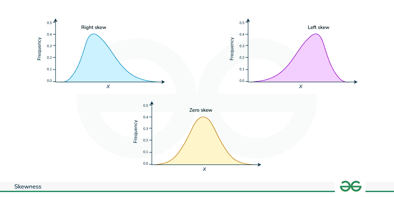
Skewness

Skewness is the measure of asymmetry of probability distribution about its mean.

Right Skew:

• Also known as positive skewness.
• Characteristics:
  • Longer or fatter tail on the right-hand side (upper tail).
  • More extreme values on the right side.
  • Mean > Median.
• Indicates a distribution that is skewed towards the left.

Left Skew:

• Also known as negative skewness.
• Characteristics:
  • Longer or fatter tail on the left-hand side (lower tail).
  • More extreme values on the left side.
  • Mean < Median.
• Indicates a distribution that is skewed towards the right.

Zero Skew:

• Also known as symmetrical distribution.
• Characteristics:
  • Symmetric distribution.
  • Left and right sides are mirror images of each other.
  • Mean = Median.
• Indicates a distribution with no skewness.

Types of Skewed data

Measure of Relationship

• Covariance: Covariance measures the degree to which two variables change together.
  [Tex]Cov(x,y) = \frac{\sum(X_i-\overline{X})(Y_i – \overline{Y})}{n} [/Tex]
• Correlation: Correlation measures the strength and direction of the linear relationship between two variables. It is represented by correlation coefficient which ranges from -1 to 1. A positive correlation indicates a direct relationship, while a negative correlation implies an inverse relationship. Pearson’s correlation coefficient is given by:
  [Tex]\rho(X, Y) = \frac{cov(X,Y)}{\sigma_X \sigma_Y} [/Tex]

Probability Theory

Here are some basic concepts or terminologies used in probability:

Term	Definition
Sample Space	The set of all possible outcomes in a probability experiment. For instance, in a coin toss, it’s “head” and “tail”.
Sample Point	One of the possible results in an experiment. For example, in rolling a fair six-sided dice, sample points are 1 to 6.
Experiment	A process or trial with uncertain results. Examples include coin tossing, card selection, or rolling a die.
Event	A subset of the sample space representing certain outcomes. Example: getting “1” when rolling a die.
Favorable Outcome	An outcome that produces the desired or expected consequence.

Various other probability formulas are,

Joint Probability (Intersection of Event)	Probability of occurring events A and B	P(A and B) = P(A) × P(B)
Union of Events	Probability of occurring events A or B	P(A or B) = P(A) + P(B) – P(A and B)
Conditional Probability	Probability of occurring events A when event B has occurred	P(A | B) = P(A and B)/P(B)

Bayes Theorem

Bayes’ Theorem is a fundamental concept in probability theory that relates conditional probabilities. It is named after the Reverend Thomas Bayes, who first introduced the theorem. Bayes’ Theorem is a mathematical formula that provides a way to update probabilities based on new evidence. The formula is as follows:

[Tex]P(A|B) = \frac{P(B|A) \times P(A)}{P(B)} [/Tex]

where

• P(A∣B): Probability of event A given that event B has occurred (posterior probability).
• P(B∣A): Probability of event B given that event A has occurred (likelihood).
• P(A): Probability of event A occurring (prior probability).
• P(B): Probability of event B occurring.

Types of Probability Functions

• Probability Mass Function(PMF)
  Probability Mass Function is a concept in probability theory that describes the probability distribution of a discrete random variable. The PMF gives the probability of each possible outcome of a discrete random variable.
• Probability Density Function (PDF)
  Probability Density Function describes the likelihood of a continuous random variable falling within a particular range. It’s the derivative of the cumulative distribution function (CDF).
• Cumulative Distribution Function (CDF)
  Cumulative Distribution Function gives the probability that a random variable will take a value less than or equal to a given value. It’s the integral of the probability density function (PDF).
• Empirical Distribution Function (EDF):
  Empirical Distribution Function is a non-parametric estimator of the cumulative distribution function (CDF) based on observed data. For a given set of data points, the EDF represents the proportion of observations less than or equal to a specific value. It is constructed by sorting the data and assigning a cumulative probability to each data point.

Probability Distributions Functions

Normal or Gaussian Distribution

The normal distribution is a continuous probability distribution characterized by its bell-shaped curve and can be by described by mean (μ) and standard deviation (σ).

Formula: [Tex]f(X|\mu,\sigma)=\frac{\epsilon^{-0.5(\frac{X-\mu}{\sigma})^2}}{\sigma\sqrt(2\pi)} [/Tex]

There is a empirical rule in normal distribution, which states that:

• Approximately 68% of the data falls within one standard deviation (σ) of the mean in both directions. This is often referred to as the 68-95-99.7 rule.
• About 95% of the data falls within two standard deviations (2σ) of the mean.
• Approximately 99.7% of the data falls within three standard deviations (3σ) of the mean.

These rule is used to detect outliers.

Central Limit Theorem

The Central Limit Theorem (CLT) states that, regardless of the shape of the original population distribution, the sampling distribution of the sample mean will be approximately normally distributed if the sample size tends to infinity.

Student t-distribution

The t-distribution, also known as Student’s t-distribution, is a probability distribution that is used in statistics.

[Tex]f(t) =\frac{\Gamma\left(\frac{df+1}{2}\right)}{\sqrt{df\pi} \, \Gamma\left(\frac{df}{2}\right)} \left(1 + \frac{t^2}{df}\right)^{-\frac{df+1}{2}} [/Tex]

where,

• Γ(.) is the gamma function
• df = Degrees of freedom 

Chi-square Distribution

The chi-squared distribution, denoted as [Tex]\chi ^2 [/Tex] is a probability distribution used in statistics it is related to the sum of squared standard normal deviates.[Tex]\chi^2 = \frac 1{2^{k/2}\Gamma {(k/2)}} x^{{\frac k 2}-1} e^{\frac {-x}2} [/Tex]

Binomial Distribution

The binomial distribution models the number of successes in a fixed number of independent Bernoulli trials, where each trial has the same probability of success (p).

Formula: [Tex]P(X=k)=(^n_k)p^k(1-p)^{n-k} [/Tex]

Assuming each trial is an independent event with a success probability of p=0.5, and we are calculating the probability of getting 3 successes in 6 trials: [Tex]P(X=3)=(^6_3)(0.5)^3(1-0.5)^3=0.3125 [/Tex]

Poisson Distribution

The Poisson distribution models the number of events that occur in a fixed interval of time or space. It’s characterized by a single parameter (λ), the average rate of occurrence.

Formula: [Tex]P(X=k)=\frac{\epsilon^{-\lambda}\lambda^k}{k!} [/Tex]

For the previous dataset, assuming the average rate of waiting time is λ=10, and we are calculating the probability of waiting exactly 12 minutes: [Tex]P(X=12)=\frac{\varepsilon^{-10}.10^{12}}{12!}≈0.0948 [/Tex]

Uniform Distribution

The uniform distribution represents a constant probability for all outcomes in a given range.

Formula: [Tex]f(X)=\frac{1}{b-a} [/Tex]

For the same previous dataset, assuming the bus arrives uniformly between 5 and 18 minutes so the probability of waiting less than 15 minutes: [Tex]P(X<15)= ∫_5^{15}\frac{1}{18-5}dx=\frac{10}{13}=0.7692 [/Tex]

Parameter estimation for Statistical Inference

• Population: Population is the group of individual, object or measurements about which you want to draw conclusion.
• Sample: Sample is the subset of population; the group chosen from the larger population to gather information and make inference about entire population.
• Expectation: Expectation, in statistics and probability theory, represents the anticipated or average value of a random variable. It is represented by E(x).
• Parameter: A parameter is a numerical characteristic of a population that is of interest in statistical analysis.
  Examples of parameters include the population mean (μ), population standard deviation (σ), or the success probability in a binomial distribution.
• Statistic: A statistic is a numerical value or measure calculated from a sample of data. It is used to estimate or infer properties of the corresponding population.
• Estimation: Estimation involves using sample data to make inferences or predictions about population parameters.
• Estimator: An estimator is a statistic used to estimate an unknown parameter in a statistical model.
• Bias: Bias in parameter estimation refers to the systematic error or deviation of the estimated value from the true value of the parameter.
  [Tex]Bias(\widehat{\theta}) = E(\widehat{\theta}) – \theta [/Tex]
  An estimator is considered unbiased if, on average, it produces parameter estimates that are equal to the true parameter value. Bias is measured as the difference between the expected value of the estimator and the true parameter value.
  [Tex]E(\widehat{\theta}) = \theta [/Tex]

Hypothesis Testing

Hypothesis testing makes inferences about a population parameter based on sample statistic.

Null Hypothesis (H₀) and Alternative Hypothesis (H₁)

• H₀ : There is no significant difference or effect.
• H₁ : There is a significant effect i.e the given statement can be false.

Degrees of freedom

Degrees of freedom (df) in statistics represent the number of values or quantities in the final calculation of a statistic that are free to vary. It is mainly defined as sample size – one(n-1).

Level of Significance([Tex]\alpha [/Tex])

This is the threshold used to determine statistical significance. Common values are 0.05, 0.01, or 0.10.

p-value

The p-value, short for probability value, is a fundamental concept in statistics that quantifies the evidence against a null hypothesis.

• If p-value ≤ α: Reject the null hypothesis.
• If p-value > α: Fail to reject the null hypothesis (meaning there isn’t enough evidence to reject it).

Type I Error and Type II Error

Type I Error that occurs when the null hypothesis is true, but the statistical test incorrectly rejects it. It is often referred to as a “false positive” or “alpha error.”

Type II Error that occurs when the null hypothesis is false, but the statistical test fails to reject it. It is often referred to as a “false negative.”

Confidence Intervals

A confidence interval is a range of values that is used to estimate the true value of a population parameter with a certain level of confidence. It provides a measure of the uncertainty or margin of error associated with a sample statistic, such as the sample mean or proportion.

Example of Hypothesis testing:

Let us consider An e-commerce company wants to assess whether a recent website redesign has a significant impact on the average time users spend on their website.

The company collects the following data:

• Data on user session durations before and after the redesign.
• Before redesign: Sample mean ([Tex]\overline{\rm x}   [/Tex]) = 3.5 minutes, Sample standard deviation (s) = 1.2 minutes, Sample size (n) = 50.
• After redesign: Sample mean ([Tex]\overline{\rm x}   [/Tex]= 4.2 minutes, Sample standard deviation (s​) = 1.5 minutes, Sample size (n) = 60.

The Hypothesis are defined as:

• Null Hypothesis (H0​): The website redesign has no impact on the average user session duration [Tex]\mu_{after} -\mu_{before} = 0 [/Tex]
• Alternative Hypothesis (Ha​): The website redesign has a positive impact on the average user session duration [Tex]\mu_{after} -\mu_{before} > 0 [/Tex]

Significance Level:

Choose a significance level, α=0.05(commonly used)

Test Statistic and P-Value:

• Conduct a test for the difference in means.
• Calculate the test statistic and p-value.

Result:

• If the p-value is less than the chosen significance level, reject the null hypothesis.
• If the p-value is greater than or equal to the significance level, fail to reject the null hypothesis.

Interpretations:

Based on the analysis, the company draws conclusions about whether the website redesign has a statistically significant impact on user session duration.

Statistical Tests:

Parametric test are statistical methods that make assumption that the data follows normal distribution.

Z-test	t-test	F-test
Testing if the mean of a sample is significantly different from a known population mean	Comparing means of two independent samples or testing if the mean of a sample is significantly different from a known or hypothesized population mean	Comparing the variances of multiple groups to assess if they are significantly different
Used when the population standard deviation is known, and the sample size is sufficiently large.	Used when the population standard deviation is unknown or when dealing with small sample sizes	Used to compare variances between two or more groups.
One-Sample Test: Z = [Tex] \frac{\overline{X}-\mu}{\frac{\sigma}{\sqrt{n}}} [/Tex] Two-Sample Test: Z = [Tex]\frac{\overline{X_1} -\overline{X_2}}{\sqrt{\frac{\sigma_{1}^{2}}{n_1} + \frac{\sigma_{2}^{2}}{n_2}}} [/Tex]	One- sample: t = [Tex]\frac{\overline{X}- \mu}{\frac{s}{\sqrt{n}}} [/Tex] Two-Sample Test: [Tex]t= \frac{\overline{X_1} – \overline{X_2}}{\sqrt{\frac{s_{1}^{2}}{n_1} + \frac{s_{2}^{2}}{n_2}}} [/Tex] Paired t-Test: t=[Tex]\frac{\overline{d}}{\frac{s_d}{\sqrt{n}}} [/Tex] d= difference	[Tex]F = \frac{s_{1}^{2}}{s_{2}^{2}}[/Tex]

ANOVA (Analysis Of Variance)

Source of Variation	Sum of Squares	Degrees Of Freedom	Mean Squares	F-Value
Between Groups	SSB= [Tex]\Sigma n _1(\bar x_1 – \bar x)^2 [/Tex]	df1=k-1	MSB= SSB/ (k-1)	f=MSB/MSE
Error	SSE=[Tex]\Sigma\Sigma (\bar x_1 – \bar x)^2 [/Tex]	df2=N-1	MSE=SSE/(N-k)
Total	SST= SSE+SSE	df3=N-1

There are mainly two types of ANOVA:

1. One-way Anova: Used to compare means of three or more groups to determine if there are statistically significant differences among them.
   here,
   • H₀​: The means of all groups are equal.
   • H₁​: At least one group mean is different.
2. Two-way Anova: It assess the influence of two categorical independent variables on a dependent variable, examining the main effects of each variable and their interaction effect.

Chi-Squared Test

The chi-squared test is a statistical test used to determine if there is a significant association between two categorical variables. It compares the observed frequencies in a contingency table with the frequencies. Formula:
[Tex]X^2=\Sigma{\frac{(O_{ij}-E_{ij})^2}{E_{ij}}}[/Tex].

This test is also performed on big data with multiple number of observations.

Non-Parametric Test

Non-parametric test does not make assumptions about the distribution of the data. They are useful when data does not meet the assumptions required for parametric tests.

• Mann-Whitney U Test: Mann-Whitney U Test is used to determine whether there is a difference between two independent groups when the dependent variable is ordinal or continuous. Applicable when assumptions for a t-test are not met. In it we rank all data points, combines the ranks, and calculates the test statistic.
• Kruskal-Wallis Test: Kruskal-Wallis Test is used to determine whether there are differences among three or more independent groups when the dependent variable is ordinal or continuous. Non-parametric alternative to one-way ANOVA.

A/B Testing or Split Testing

A/B testing, also known as split testing, is a method used to compare two versions (A and B) of a webpage, app, or marketing asset to determine which one performs better.

Example : a product manager change a website’s “Shop Now” button color from green to blue to improve the click-through rate (CTR). Formulating null and alternative hypotheses, users are divided into A and B groups, and CTRs are recorded. Statistical tests like chi-square or t-test are applied with a 5% confidence interval. If the p-value is below 5%, the manager may conclude that changing the button color significantly affects CTR, informing decisions for permanent implementation.

Regression

Regression is a statistical technique used to model the relationship between a dependent variable and one or more independent variables.

The equation for regression: 
[Tex]y=\alpha+ \beta x[/Tex]

Where,

• y is the dependent variable,
• x is the independent variable
• [Tex]\alpha[/Tex] is the intercept
• [Tex]\beta[/Tex] is the regression coefficient.

Regression coefficient is a measure of the strength and direction of the relationship between a predictor variable (independent variable) and the response variable (dependent variable).
[Tex]\beta = \frac{\sum(X_i-\overline{X})(Y_i – \overline{Y})}{\sum(X_i-\overline{X})^2}[/Tex]

Conclusion

In summary, statistics is a vital tool for understanding and utilizing data across various fields. Descriptive statistics simplify and organize data, while inferential statistics allow us to draw conclusions and make predictions based on samples. Measures like central tendency, dispersion, and shape offer insights into data characteristics. Hypothesis testing, confidence intervals, and probability distributions help make informed decisions and analyze relationships between variables. Whether you’re preparing for an interview, exploring data science, or making business choices, a solid grasp of statistics is essential for success in navigating and interpreting the complexities of data.

Statistics Cheat Sheet – FAQs

Is this cheat sheet suitable for Class 10 students?

Yes, this cheat sheet simplifies statistics concepts for easy understanding, suitable for Class 10 students.

Can this Statistics cheat sheets help in machine learning?

Yes, absolutely! Statistics is foundational to machine learning

What are the top 5 fundamental statistics formulas?

Top 5 Fundamental Stats Formulas:

1. Mean (average): Σxᵢ / n (numerical data)
2. Median: Middle value (ordered data)
3. Standard deviation: √(Σ(xᵢ – mean)² / (n – 1)) (numerical data)
4. Probability: Favorable outcomes / Total possible outcomes
5. Sample proportion: p = x / n (categorical data)