DeepAR Forecasting Algorithm

In the field of time series forecasting, where the ability to predict future values based on historical data is crucial, advanced machine learning algorithms have become indispensable. One such powerful algorithm is DeepAR, which has gained prominence for its effectiveness in handling complex temporal patterns and generating accurate forecasts. DeepAR is particularly well-suited for scenarios where multiple related time series need to be forecasted simultaneously, making it a valuable tool in various domains like finance, e-commerce, and supply chain management. In this article, we will discuss about DeepAR forecasting algorithm and implement it for time-series forecasting.

What is DeepAR?

For advanced time-series forecasting, Amazon Corporation developed a state-of-the-art probabilistic forecasting algorithm which is known as the Deep Autoregressive or DeepAR forecasting algorithm. This is one kind of Deep Learning model that is specifically designed to capture the inherent uncertainties associated with future predictions. Unlike traditional forecasting methods that rely on deterministic point estimates, DeepAR provides a probability distribution over future values, allowing decision-makers to assess the range of possible outcomes and make more informed decisions.

Working principals of DeepAR

There are some key-working principals of DeepAR is listed below:

1. Autoregressive Architecture: DeepAR employs an autoregressive neural network architecture, where the predictions for each time step depend on a combination of historical observations and the model’s own past predictions. This enables the algorithm to capture more complex dependencies within the time series data, making it adept at handling sequences with intricate patterns and trends.
2. Embedding of Categorical Features: DeepAR can seamlessly incorporate information from categorical features associated with time series data. This is achieved through the use of embeddings, which transform categorical variables into continuous vectors. The inclusion of such features enhances the model’s ability to discern patterns and relationships within the data, especially in scenarios where external factors influence the time series.
3. Temporal Attention Mechanism: To effectively weigh the importance of different time points in the historical data, DeepAR utilizes a temporal attention mechanism. This mechanism enables the model to focus on relevant portions of the time series, adapting its attention dynamically based on the patterns present in the data.
4. Training with Quantile Loss: DeepAR is trained using a probabilistic approach that minimizes the quantile loss. This means the model is optimized to generate prediction intervals, representing the range of possible future values with associated confidence levels. This probabilistic framework is particularly valuable in decision-making processes, providing decision-makers with a nuanced understanding of the uncertainty associated with the forecasts.

DeepAR Forecast Step-by-step implementation

Installing required modules

At first, we will install all required Python modules to our runtime.

!pip install gluonts
!pip install --upgrade mxnet==1.6.0
!pip install "gluonts[torch]"

Importing required libraries

Now we will import all required Python libraries like NumPy, Pandas, Matplotlib and OS etc.

Python3

import numpy as np
import pandas as pd
import os
import matplotlib as mpl
import matplotlib.pyplot as plt
from gluonts.torch.model.deepar import DeepAREstimator
from gluonts.dataset.common import ListDataset
from gluonts.dataset.field_names import FieldName
from gluonts.evaluation.backtest import make_evaluation_predictions
from tqdm.autonotebook import tqdm
from gluonts.evaluation import Evaluator
from typing import Dict

Dataset loading and pre-processing

Now we will load two simple datasets as DeepAR is mainly use for multiple time-series forecasting. Both the datasets can be downloaded from here: dataset1 and dataset2. After that, we will slice the datasets to make them equally distributed and merge them. Then the merged dataset will be split into training and testing sets.

Python3

# https://www.kaggle.com/datasets/robikscube/hourly-energy-consumption/data?select=COMED_hourly.csv
df_comed = pd.read_csv("/content/COMED_hourly.csv", parse_dates=True)
# https://www.kaggle.com/datasets/robikscube/hourly-energy-consumption/data?select=DOM_hourly.csv
df_dom = pd.read_csv("/content/DOM_hourly.csv", parse_dates=True)
# Slicing the datasets to make equal lengh data
df_comed = df_comed.loc[df_comed["Datetime"]
                        > '2011-12-31'].reset_index(drop=True)
df_dom = df_dom.loc[df_dom["Datetime"] > '2011-12-31'].reset_index(drop=True)
df_comed = df_comed.T
df_comed.columns = df_comed.iloc[0]
df_comed = df_comed.drop(df_comed.index[0])
df_comed['Station_Name'] = "COMED"
df_comed = df_comed.reset_index(drop=True)
df_dom = df_dom.T
df_dom.columns = df_dom.iloc[0]
df_dom = df_dom.drop(df_dom.index[0])
df_dom['Station_Name'] = "DOM"
df_dom = df_dom.reset_index(drop=True)
df_all = pd.concat([df_comed, df_dom], axis=0)
df_all = df_all.set_index("Station_Name")
df_all = df_all.reset_index()

ts_code = df_all['Station_Name'].astype('category').cat.codes.values
freq = "1H"  # rate at  which dataset is sampled
start_train = pd.Timestamp("2011-12-31 01:00:00", freq=freq)
start_test = pd.Timestamp("2016-06-10 18:00:00", freq=freq)
prediction_lentgh = 24 * 1  # Our prediction Length is 1 Day
# training and testing sets split
df_train = df_all.iloc[:, 1:40000].values
df_test = df_all.iloc[:, 40000:].values

You can securely ignore all warnings.

Model defining

Now we will initialize the DeepAR estimator model by defining its various hyper-parameters which are listed below–>

• freq: this parameter defines the frequency of the time series data. It represents the number of time steps in one period or cycle of the time series. Our data has daily observations, so, the frequency is determined by the variable freq.
• context_length: This parameter sets the number of time steps that the model uses to learn patterns and dependencies in the historical data. Here it is set to (24 * 5), indicating that the model looks back over a period equivalent to 5 days (by assuming each time step corresponds to an hour).
• prediction_length: This parameter specifies how far into the future the model should generate predictions. It determines the length of the forecast horizon.
• cardinality: This parameter is a list that indicates the number of categories for each categorical feature in the dataset.
• num_layers: It determines the number of layers in the neural network architecture. In our case, the model is configured with 2 layers.
• dropout_rate: It is a regularization technique that helps prevent overfitting. It represents the fraction of input units to drop out during training. A value of 0.25 means that 25% of the input units will be randomly set to zero during each update.
• trainer_kwargs: This is a dictionary containing additional arguments for the training process. In our case, it includes 'max_epochs': 16, which sets the maximum number of training epochs. An epoch is one complete pass through the entire training dataset.

Python3

estimator = DeepAREstimator(freq=freq,
                            # context length is number of time steps will look back(5 days in a week)
                            context_length=24 * 5,
                            prediction_length=prediction_lentgh,
                            cardinality=[1],
                            num_layers=2,
                            dropout_rate=0.25,
                            trainer_kwargs={'max_epochs': 16}
                            )

Dataset preparation

For every deep learning model, it is required to prepare the raw dataset as per model’s input type. Here also, we need to redefine our raw dataset for training and testing.

Python3

train_ds = ListDataset([
    {
        FieldName.TARGET: target,
        FieldName.START: start_train,
        FieldName.FEAT_STATIC_CAT: fsc
    }
    for (target, fsc) in zip(df_train,
                             ts_code.reshape(-1, 1))
], freq=freq)

test_ds = ListDataset([
    {
        FieldName.TARGET: target,
        FieldName.START: start_test,
        FieldName.FEAT_STATIC_CAT: fsc
    }
    for (target, fsc) in zip(df_test,
                             ts_code.reshape(-1, 1))
], freq=freq)

Model Training

Now we are ready to train the DeepAR estimator by passing the training dataset which is just prepared. Here we will utilize four CPU code as workers for fast processing.

Python3

predictor = estimator.train(training_data=train_ds, num_workers=4)

Forecasting

So, training is completed. Now our task is simply plot the forecasted values with actual. DeepAR supports confidence interval values so we will take the median of forecast to make the closest prediction. In the plot, the gap between the actual and forecasted lines is the confidence zone(like 75% or 90% confidence of prediction etc.).

Python3

forecast_it, ts_it = make_evaluation_predictions(
    dataset=test_ds,
    predictor=predictor,
    num_samples=100,
)

print("Gathering time series conditioning values ...")
tss = list(tqdm(ts_it, total=len(df_test)))
print("Gathering time series predictions ...")
forecasts = list(tqdm(forecast_it, total=len(df_test)))


def plot_prob_forecasts(ts_entry, forecast_entry):
    plot_length = prediction_lentgh
    prediction_intervals = (0.5, 0.8)
    legend = ["observations", "median prediction"] + \
        [f"{k*100}% prediction interval" for k in prediction_intervals][::-1]

    fig, ax = plt.subplots(1, 1, figsize=(10, 7))
    ts_entry[-plot_length:].plot(ax=ax, color='blue', label='observations')

    # Extract the median prediction
    median = np.median(forecast_entry, axis=0)
    ax.plot(ts_entry.index[-plot_length:], median[-plot_length:],
            color='orange', label='median prediction')

    # Extract the prediction intervals if available
    if len(forecast_entry) > 1:
        lower, upper = np.percentile(forecast_entry, q=[(1 - k) * 100 / 2 for k in prediction_intervals], axis=0), np.percentile(
            forecast_entry, q=[(1 + k) * 100 / 2 for k in prediction_intervals], axis=0)

        # Ensure lower and upper are 1-D arrays
        lower, upper = lower[-plot_length:], upper[-plot_length:]

    plt.grid(which="both")
    plt.legend(legend, loc="upper left")
    plt.show()


for i in tqdm(range(2)):
    ts_entry = tss[i]
    forecast_entry = np.array(forecasts[i].samples)
    plot_prob_forecasts(ts_entry, forecast_entry)

Output:

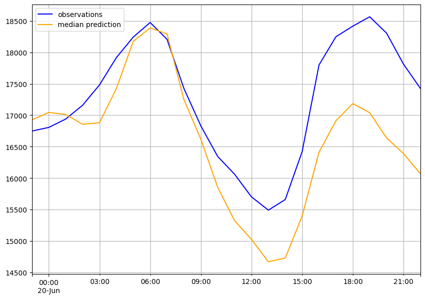
Actual vs. forecasted values

The 2nd plot is to be considered as more we iterate more accurate it will be.

Evaluations

DeepAR itself provides a wide range of performance metrics like quantile loss, MAPE etc.

Python3

evaluator = Evaluator(quantiles=[0.1, 0.5, 0.9])
agg_metrics, item_metrics = evaluator(iter(tss), iter(forecasts), num_series=len(df_test))
item_metrics

Output:

item_id    forecast_start    MSE    abs_error    abs_target_sum    abs_target_mean    seasonal_error    MASE    MAPE    sMAPE    num_masked_target_values    ND    MSIS    QuantileLoss[0.1]    Coverage[0.1]    QuantileLoss[0.5]    Coverage[0.5]    QuantileLoss[0.9]    Coverage[0.9]
0    None    2018-06-19 23:00    318517.437500    11284.473633    297067.0    12377.791667    777.236948    0.604946    0.038610    0.037733    0.0    0.037986    3.896573    3385.887109    0.041667    11284.473633    0.583333    6079.214258    1.000000
1    None    2018-06-19 23:00    835246.333333    16977.113281    414494.0    17270.583333    909.647006    0.777642    0.040786    0.042074    0.0    0.040959    4.620998    9115.450977    0.000000    16977.114258    0.166667    6252.767773    0.708333

So, we can see that the errors are significantly low for every case.

Conclusion

We can conclude that DeepAR is an effective deep learning model for forecasting problems. However, for more accurate forecasting it required to train the model in more epochs.