Evaluation Metrics in Machine Learning

Evaluation is always good in any field, right? In the case of machine learning, it is best practice. In this post, we will almost cover all the popular as well as common metrics used for machine learning.

Classification Metrics

In a classification task, our main task is to predict the target variable which is in the form of discrete values. To evaluate the performance of such a model there are metrics as mentioned below:

• Classification Accuracy
• Logarithmic loss
• Area under Curve
• F1 score
  • Precision
  • Recall
• Confusion Matrix

Classification Accuracy

Classification accuracy is the accuracy we generally mean, whenever we use the term accuracy. We calculate this by calculating the ratio of correct predictions to the total number of input Samples.

It works great if there are an equal number of samples for each class. For example, we have a 90% sample of class A and a 10% sample of class B in our training set. Then, our model will predict with an accuracy of 90% by predicting all the training samples belonging to class A. If we test the same model with a test set of 60% from class A and 40% from class B. Then the accuracy will fall, and we will get an accuracy of 60%. 

Classification accuracy is good but it gives a False Positive sense of achieving high accuracy. The problem arises due to the possibility of misclassification of minor class samples being very high. 

Logarithmic Loss

It is also known as Log loss. Its basic working propaganda is by penalizing the false (False Positive) classification. It usually works well with multi-class classification. Working on Log loss, the classifier should assign a probability for each and every class of all the samples. If there are N  samples belonging to the M class, then we calculate the Log loss in this way:

Now the Terms, 

• y_ij indicate whether sample i belongs to class j.
• p_ij – The probability of sample i belongs to class j.
• The range of log loss is [0,?). When the log loss is near 0 it indicates high accuracy and when away from zero then, it indicates lower accuracy.
• Let me give you a bonus point, minimizing log loss gives you higher accuracy for the classifier.

Area Under Curve(AUC)

It is one of the widely used metrics and basically used for binary classification. The AUC of a classifier is defined as the probability of a classifier will rank a randomly chosen positive example higher than a negative example. Before going into  AUC  more, let me make you comfortable with a few basic terms. 

True positive rate:

Also called or termed sensitivity. True Positive Rate is considered as a portion of positive data points that are correctly considered as positive, with respect to all data points that are positive.

True Negative Rate

Also called or termed specificity. False Negative Rate is considered as a portion of negative data points that are correctly considered as negative, with respect to all data points that are negatives.

False-positive Rate

False Negative Rate is considered as a portion of negative data points that are mistakenly considered as negative, with respect to all data points that are negative.

False Positive Rate and True Positive Rate both have values in the range [0, 1]. Now the thing is what is A U C then? So, A U C  is a curve plotted between False Positive Rate Vs True Positive Rate at all different data points with a range of  [0, 1]. Greater the value of AUCC better the performance of the model.

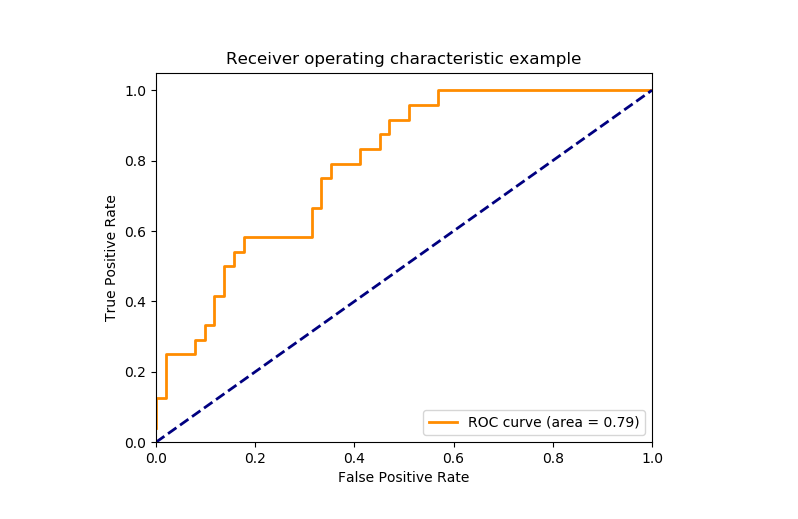
ROC Curve for Evaluation of Classification Models

F1 Score

It is a harmonic mean between recall and precision. Its range is [0,1]. This metric usually tells us how precise (It correctly classifies how many instances) and robust (does not miss any significant number of instances) our classifier is. 

Precision

There is another metric named Precision. Precision is a measure of a model’s performance that tells you how many of the positive predictions made by the model are actually correct. It is calculated as the number of true positive predictions divided by the number of true positive and false positive predictions.

Recall

Lower recall and higher precision give you great accuracy but then it misses a large number of instances. The more the F1 score better will be performance. It can be expressed mathematically in this way:

Confusion Matrix

It creates a N X N matrix, where N is the number of classes or categories that are to be predicted. Here we have N = 2, so we get a 2 X 2 matrix. Suppose there is a problem with our practice which is a binary classification. Samples of that classification belong to either Yes or No. So, we build our classifier which will predict the class for the new input sample. After that, we tested our model with 165 samples, and we get the following result.

There are 4 terms you should keep in mind:

1. True Positives: It is the case where we predicted Yes and the real output was also yes.
2. True Negatives: It is the case where we predicted No and the real output was also No.
3. False Positives: It is the case where we predicted Yes but it was actually No.
4. False Negatives: It is the case where we predicted No but it was actually Yes. 

The accuracy of the matrix is always calculated by taking average values present in the main diagonal i.e.

Regression Evaluation Metrics

In the regression task, we are supposed to predict the target variable which is in the form of continuous values. To evaluate the performance of such a model below mentioned evaluation metrics are used:

• Mean Absolute Error
• Mean Squared Error
• Root Mean Square Error
• Root Mean Square Logarithmic Error
• R2 – Score

Mean Absolute Error(MAE)

It is the average distance between Predicted and original values. Basically, it gives how we have predicted from the actual output. However, there is one limitation i.e. it doesn’t give any idea about the direction of the error which is whether we are under-predicting or over-predicting our data. It can be represented mathematically in this way:

Mean Squared Error(MSE)

It is similar to mean absolute error but the difference is it takes the square of the average of between predicted and original values. The main advantage to take this metric is here, it is easier to calculate the gradient whereas, in the case of mean absolute error, it takes complicated programming tools to calculate the gradient. By taking the square of errors it pronounces larger errors more than smaller errors, we can focus more on larger errors. It can be expressed mathematically in this way.

Root Mean Square Error(RMSE)

We can say that RMSE is a metric that can be obtained by just taking the square root of the MSE value. As we know that the MSE metrics are not robust to outliers and so are the RMSE values. This gives higher weightage to the large errors in predictions.

Root Mean Squared Logarithmic Error(RMSLE)

There are times when the target variable varies in a wide range of values. And hence we do not want to penalize the overestimation of the target values but penalize the underestimation of the target values. For such cases, RMSLE is used as an evaluation metric which helps us to achieve the above objective.

Some changes in the original formula of the RMSE code will give us the RMSLE formula that is as shown below:

R2 – Score

The coefficient of determination also called the R2 score is used to evaluate the performance of a linear regression model. It is the amount of variation in the output-dependent attribute which is predictable from the input independent variable(s). It is used to check how well-observed results are reproduced by the model, depending on the ratio of total deviation of results described by the model.