Getting Started with Python OpenCV

Computer Vision is one of the techniques from which we can understand images and videos and can extract information from them. It is a subset of artificial intelligence that collects information from digital images or videos. 

Python OpenCV is the most popular computer vision library. By using it, one can process images and videos to identify objects, faces, or even handwriting of a human. When it is integrated with various libraries, such as NumPy, python is capable of processing the OpenCV array structure for analysis.

In this article, we will discuss Python OpenCV in detail along with some common operations like resizing, cropping, reading, saving images, etc with the help of good examples.

Installation

To install OpenCV, one must have Python and PIP, preinstalled on their system. If Python is not present, go through How to install Python on Linux? and follow the instructions provided. If PIP is not present, go through How to install PIP on Linux? and follow the instructions provided.

After installing both Python and PIP, type the below command in the terminal.

pip3 install opencv-python

Reading Images

To read the images cv2.imread() method is used. This method loads an image from the specified file. If the image cannot be read (because of the missing file, improper permissions, unsupported or invalid format) then this method returns an empty matrix.

Image Used:

Example: Python OpenCV Read Image

Python3

# Python code to read image
import cv2

# To read image from disk, we use
# cv2.imread function, in below method,
img = cv2.imread("geeks.png", cv2.IMREAD_COLOR)

print(img)

Output:

[[[ 87 157  14]
  [ 87 157  14]
  [ 87 157  14]
  ...
  [ 87 157  14]
  [ 87 157  14]
  [ 87 157  14]]

 [[ 87 157  14]
  [ 87 157  14]
  [ 87 157  14]
  ...
  [ 87 157  14]
  [ 87 157  14]
  [ 87 157  14]]

 [[ 87 157  14]
  [ 87 157  14]
  [ 87 157  14]
  ...
  [ 87 157  14]
  [ 87 157  14]
  [ 87 157  14]]

 ...

 [[ 72 133   9]
  [ 72 133   9]
  [ 72 133   9]
  ...
  [ 87 157  14]
  [ 87 157  14]
  [ 87 157  14]]

 [[ 72 133   9]
  [ 72 133   9]
  [ 72 133   9]
  ...
  [ 87 157  14]
  [ 87 157  14]
  [ 87 157  14]]

 [[ 72 133   9]
  [ 72 133   9]
  [ 72 133   9]
  ...
  [ 87 157  14]
  [ 87 157  14]
  [ 87 157  14]]]

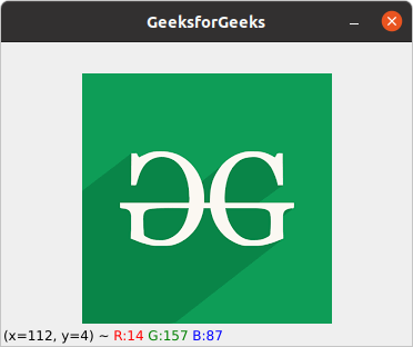
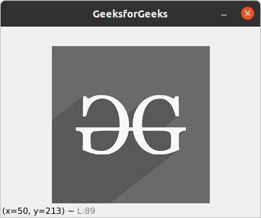
Displaying Images

cv2.imshow() method is used to display an image in a window. The window automatically fits the image size.

Example: Python OpenCV Display Images

Python3

# Python code to read image
import cv2

# To read image from disk, we use
# cv2.imread function, in below method,
img = cv2.imread("geeks.png", cv2.IMREAD_COLOR)

# Creating GUI window to display an image on screen
# first Parameter is windows title (should be in string format)
# Second Parameter is image array
cv2.imshow("GeeksforGeeks", img)

# To hold the window on screen, we use cv2.waitKey method
# Once it detected the close input, it will release the control
# To the next line
# First Parameter is for holding screen for specified milliseconds
# It should be positive integer. If 0 pass an parameter, then it will
# hold the screen until user close it.
cv2.waitKey(0)

# It is for removing/deleting created GUI window from screen
# and memory
cv2.destroyAllWindows()

Output:

Saving Images

cv2.imwrite() method is used to save an image to any storage device. This will save the image according to the specified format in the current working directory.

Example: Python OpenCV Save Images

Python3

# Python program to explain cv2.imwrite() method

# importing cv2
import cv2

image_path = 'geeks.png'

# Using cv2.imread() method
# to read the image
img = cv2.imread(image_path)

# Filename
filename = 'savedImage.jpg'

# Using cv2.imwrite() method
# Saving the image
cv2.imwrite(filename, img)

# Reading and showing the saved image
img = cv2.imread(filename)
cv2.imshow("GeeksforGeeks", img)

cv2.waitKey(0)
cv2.destroyAllWindows()

Output:

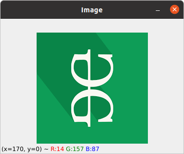
Rotating Images

cv2.rotate() method is used to rotate a 2D array in multiples of 90 degrees. The function cv::rotate rotates the array in three different ways.

Example: Python OpenCV Rotate Image

Python3

# Python program to explain cv2.rotate() method

# importing cv2
import cv2

# path
path = 'geeks.png'

# Reading an image in default mode
src = cv2.imread(path)

# Window name in which image is displayed
window_name = 'Image'

# Using cv2.rotate() method
# Using cv2.ROTATE_90_CLOCKWISE rotate
# by 90 degrees clockwise
image = cv2.rotate(src, cv2.cv2.ROTATE_90_CLOCKWISE)

# Displaying the image
cv2.imshow(window_name, image)
cv2.waitKey(0)

Output:

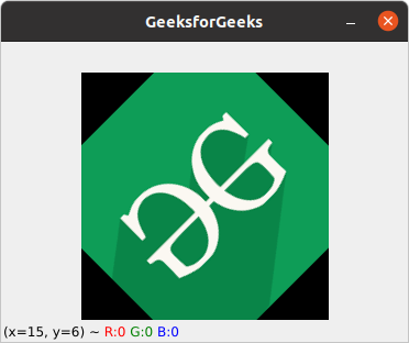
The above functions restrict us to rotate the image in the multiple of 90 degrees only. We can also rotate the image to any angle by defining the rotation matrix listing rotation point, degree of rotation, and the scaling factor.

Example: Python OpenCV Rotate Image by any Angle

Python3

import cv2
import numpy as np

FILE_NAME = 'geeks.png'

# Read image from the disk.
img = cv2.imread(FILE_NAME)

# Shape of image in terms of pixels.
(rows, cols) = img.shape[:2]

# getRotationMatrix2D creates a matrix needed
# for transformation. We want matrix for rotation
# w.r.t center to 45 degree without scaling.
M = cv2.getRotationMatrix2D((cols / 2, rows / 2), 45, 1)
res = cv2.warpAffine(img, M, (cols, rows))

cv2.imshow("GeeksforGeeks", res)

cv2.waitKey(0)
cv2.destroyAllWindows()

Output:

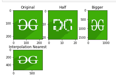
Resizing Image

Image resizing refers to the scaling of images. It helps in reducing the number of pixels from an image and that has several advantages e.g. It can reduce the time of training of a neural network as more is the number of pixels in an image more is the number of input nodes that in turn increases the complexity of the model. It also helps in zooming in images. Many times we need to resize the image i.e. either shrink it or scale up to meet the size requirements.

OpenCV provides us with several interpolation methods for resizing an image. Choice of Interpolation Method for Resizing –

• cv2.INTER_AREA: This is used when we need to shrink an image.
• cv2.INTER_CUBIC: This is slow but more efficient.
• cv2.INTER_LINEAR: This is primarily used when zooming is required. This is the default interpolation technique in OpenCV.

Example: Python OpenCV Image Resizing

Python3

import cv2
import numpy as np
import matplotlib.pyplot as plt

image = cv2.imread("geeks.png", 1)
# Loading the image

half = cv2.resize(image, (0, 0), fx = 0.1, fy = 0.1)
bigger = cv2.resize(image, (1050, 1610))

stretch_near = cv2.resize(image, (780, 540),
            interpolation = cv2.INTER_NEAREST)


Titles =["Original", "Half", "Bigger", "Interpolation Nearest"]
images =[image, half, bigger, stretch_near]
count = 4

for i in range(count):
    plt.subplot(2, 3, i + 1)
    plt.title(Titles[i])
    plt.imshow(images[i])

plt.show()

Output:

Color Spaces

Color spaces are a way to represent the color channels present in the image that gives the image that particular hue. There are several different color spaces and each has its own significance. Some of the popular color spaces are RGB (Red, Green, Blue), CMYK (Cyan, Magenta, Yellow, Black), HSV (Hue, Saturation, Value), etc.

 cv2.cvtColor() method is used to convert an image from one color space to another. There are more than 150 color-space conversion methods available in OpenCV.

Example: Python OpenCV Color Spaces

Python3

# Python program to explain cv2.cvtColor() method

# importing cv2
import cv2

# path
path = 'geeks.png'

# Reading an image in default mode
src = cv2.imread(path)

# Window name in which image is displayed
window_name = 'GeeksforGeeks'

# Using cv2.cvtColor() method
# Using cv2.COLOR_BGR2GRAY color space
# conversion code
image = cv2.cvtColor(src, cv2.COLOR_BGR2GRAY )

# Displaying the image
cv2.imshow(window_name, image)

cv2.waitKey(0)
cv2.destroyAllWindows()

Output:

Arithmetic Operations

Arithmetic Operations like Addition, Subtraction, and Bitwise Operations(AND, OR, NOT, XOR) can be applied to the input images. These operations can be helpful in enhancing the properties of the input images. Image arithmetics are important for analyzing the input image properties. The operated images can be further used as an enhanced input image, and many more operations can be applied for clarifying, thresholding, dilating, etc of the image.

Addition of Image:

We can add two images by using function cv2.add(). This directly adds up image pixels in the two images. But adding the pixels is not an ideal situation. So, we use cv2.addweighted(). Remember, both images should be of equal size and depth.

Input Image1:

Input Image2:

Python3

# Python program to illustrate
# arithmetic operation of
# addition of two images

# organizing imports
import cv2
import numpy as np

# path to input images are specified and
# images are loaded with imread command
image1 = cv2.imread('star.jpg')
image2 = cv2.imread('dot.jpg')

# cv2.addWeighted is applied over the
# image inputs with applied parameters
weightedSum = cv2.addWeighted(image1, 0.5, image2, 0.4, 0)

# the window showing output image
# with the weighted sum
cv2.imshow('Weighted Image', weightedSum)

# De-allocate any associated memory usage
if cv2.waitKey(0) & 0xff == 27:
    cv2.destroyAllWindows()

Output:

Subtraction of Image:

Just like in addition, we can subtract the pixel values in two images and merge them with the help of cv2.subtract(). The images should be of equal size and depth.

Python3

# Python program to illustrate
# arithmetic operation of
# subtraction of pixels of two images

# organizing imports
import cv2
import numpy as np

# path to input images are specified and
# images are loaded with imread command
image1 = cv2.imread('star.jpg')
image2 = cv2.imread('dot.jpg')

# cv2.subtract is applied over the
# image inputs with applied parameters
sub = cv2.subtract(image1, image2)

# the window showing output image
# with the subtracted image
cv2.imshow('Subtracted Image', sub)

# De-allocate any associated memory usage
if cv2.waitKey(0) & 0xff == 27:
    cv2.destroyAllWindows()

Output:

Bitwise Operations on Binary Image

Bitwise operations are used in image manipulation and used for extracting essential parts in the image. Bitwise operations used are :

• AND
• OR
• XOR
• NOT

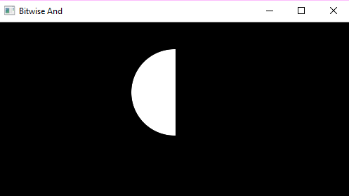
Bitwise AND operation

Bit-wise conjunction of input array elements. 

Input Image 1:

Input Image 2: 

Python3

# Python program to illustrate
# arithmetic operation of
# bitwise AND of two images

# organizing imports
import cv2
import numpy as np

# path to input images are specified and
# images are loaded with imread command
img1 = cv2.imread('input1.png')
img2 = cv2.imread('input2.png')

# cv2.bitwise_and is applied over the
# image inputs with applied parameters
dest_and = cv2.bitwise_and(img2, img1, mask = None)

# the window showing output image
# with the Bitwise AND operation
# on the input images
cv2.imshow('Bitwise And', dest_and)

# De-allocate any associated memory usage
if cv2.waitKey(0) & 0xff == 27:
    cv2.destroyAllWindows()

Output:

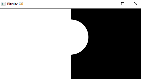
Bitwise OR operation

Bit-wise disjunction of input array elements. 

Python3

# Python program to illustrate
# arithmetic operation of
# bitwise OR of two images

# organizing imports
import cv2
import numpy as np

# path to input images are specified and
# images are loaded with imread command
img1 = cv2.imread('input1.png')
img2 = cv2.imread('input2.png')

# cv2.bitwise_or is applied over the
# image inputs with applied parameters
dest_or = cv2.bitwise_or(img2, img1, mask = None)

# the window showing output image
# with the Bitwise OR operation
# on the input images
cv2.imshow('Bitwise OR', dest_or)

# De-allocate any associated memory usage
if cv2.waitKey(0) & 0xff == 27:
    cv2.destroyAllWindows()

Output:

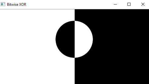
Bitwise XOR operation

Bit-wise exclusive-OR operation on input array elements. 

Python3

# Python program to illustrate
# arithmetic operation of
# bitwise XOR of two images

# organizing imports
import cv2
import numpy as np

# path to input images are specified and
# images are loaded with imread command
img1 = cv2.imread('input1.png')
img2 = cv2.imread('input2.png')

# cv2.bitwise_xor is applied over the
# image inputs with applied parameters
dest_xor = cv2.bitwise_xor(img1, img2, mask = None)

# the window showing output image
# with the Bitwise XOR operation
# on the input images
cv2.imshow('Bitwise XOR', dest_xor)

# De-allocate any associated memory usage
if cv2.waitKey(0) & 0xff == 27:
    cv2.destroyAllWindows()

Output:

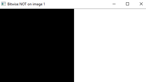
Bitwise NOT operation

Inversion of input array elements. 

Python3

# Python program to illustrate
# arithmetic operation of
# bitwise NOT on input image

# organizing imports
import cv2
import numpy as np

# path to input images are specified and
# images are loaded with imread command
img1 = cv2.imread('input1.png')
img2 = cv2.imread('input2.png')

# cv2.bitwise_not is applied over the
# image input with applied parameters
dest_not1 = cv2.bitwise_not(img1, mask = None)
dest_not2 = cv2.bitwise_not(img2, mask = None)

# the windows showing output image
# with the Bitwise NOT operation
# on the 1st and 2nd input image
cv2.imshow('Bitwise NOT on image 1', dest_not1)
cv2.imshow('Bitwise NOT on image 2', dest_not2)

# De-allocate any associated memory usage
if cv2.waitKey(0) & 0xff == 27:
    cv2.destroyAllWindows()

Output:

Bitwise NOT on Image 1 

Bitwise NOT on Image 2 

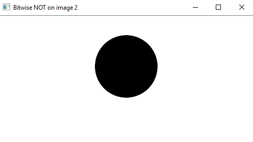
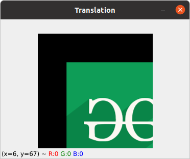
Image Translation

Translation refers to the rectilinear shift of an object i.e. an image from one location to another. If we know the amount of shift in horizontal and the vertical direction, say (tx, ty) then we can make a transformation matrix. Now, we can use the cv2.wrapAffine() function to implement the translations. This function requires a 2×3 array. The numpy array should be of float type.

Example: Python OpenCV Image Translation

Python3

import cv2
import numpy as np

image = cv2.imread('geeks.png')

# Store height and width of the image
height, width = image.shape[:2]

quarter_height, quarter_width = height / 4, width / 4

T = np.float32([[1, 0, quarter_width], [0, 1, quarter_height]])

# We use warpAffine to transform
# the image using the matrix, T
img_translation = cv2.warpAffine(image, T, (width, height))

cv2.imshow('Translation', img_translation)
cv2.waitKey(0)

cv2.destroyAllWindows()

Output:

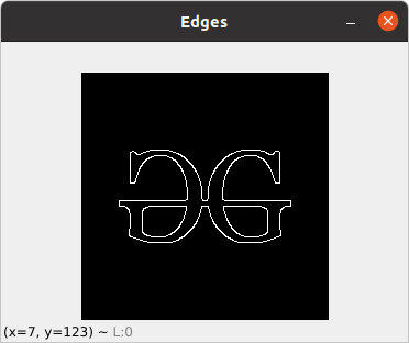
Edge Detection

The process of image detection involves detecting sharp edges in the image. This edge detection is essential in the context of image recognition or object localization/detection. There are several algorithms for detecting edges due to its wide applicability. We’ll be using one such algorithm known as Canny Edge Detection. 

Example: Python OpenCV Canny Edge Detection

Python3

import cv2

FILE_NAME = 'geeks.png'

# Read image from disk.
img = cv2.imread(FILE_NAME)

# Canny edge detection.
edges = cv2.Canny(img, 100, 200)

# Write image back to disk.
cv2.imshow('Edges', edges)
cv2.waitKey(0)
cv2.destroyAllWindows()

Output:

Simple Thresholding

Thresholding is a technique in OpenCV, which is the assignment of pixel values in relation to the threshold value provided. In thresholding, each pixel value is compared with the threshold value. If the pixel value is smaller than the threshold, it is set to 0, otherwise, it is set to a maximum value (generally 255). Thresholding is a very popular segmentation technique, used for separating an object considered as a foreground from its background. A threshold is a value that has two regions on either side i.e. below the threshold or above the threshold.

In Computer Vision, this technique of thresholding is done on grayscale images. So initially, the image has to be converted in grayscale color space.

If f (x, y) < T
  then f (x, y) = 0
else
  f (x, y) = 255

where
f (x, y) = Coordinate Pixel Value
T = Threshold Value.

In OpenCV with Python, the function cv2.threshold is used for thresholding.

The basic Thresholding technique is Binary Thresholding. For every pixel, the same threshold value is applied. If the pixel value is smaller than the threshold, it is set to 0, otherwise, it is set to a maximum value. The different Simple Thresholding Techniques are:

• cv2.THRESH_BINARY: If pixel intensity is greater than the set threshold, the value set to 255, else set to 0 (black).
• cv2.THRESH_BINARY_INV: Inverted or Opposite case of cv2.THRESH_BINARY.
• cv.THRESH_TRUNC: If pixel intensity value is greater than the threshold, it is truncated to the threshold. The pixel values are set to be the same as the threshold. All other values remain the same.
• cv.THRESH_TOZERO: Pixel intensity is set to 0, for all the pixels intensity, less than the threshold value.
• cv.THRESH_TOZERO_INV: Inverted or Opposite case of cv2.THRESH_TOZERO.

Example: Python OpenCV Simple Thresholding

Python3

# Python program to illustrate
# simple thresholding type on an image

# organizing imports
import cv2
import numpy as np

# path to input image is specified and
# image is loaded with imread command
image1 = cv2.imread('geeks.png')

# cv2.cvtColor is applied over the
# image input with applied parameters
# to convert the image in grayscale
img = cv2.cvtColor(image1, cv2.COLOR_BGR2GRAY)

# applying different thresholding
# techniques on the input image
# all pixels value above 120 will
# be set to 255
ret, thresh1 = cv2.threshold(img, 120, 255, cv2.THRESH_BINARY)
ret, thresh2 = cv2.threshold(img, 120, 255, cv2.THRESH_BINARY_INV)
ret, thresh3 = cv2.threshold(img, 120, 255, cv2.THRESH_TRUNC)
ret, thresh4 = cv2.threshold(img, 120, 255, cv2.THRESH_TOZERO)
ret, thresh5 = cv2.threshold(img, 120, 255, cv2.THRESH_TOZERO_INV)

# the window showing output images
# with the corresponding thresholding
# techniques applied to the input images
cv2.imshow('Binary Threshold', thresh1)
cv2.imshow('Binary Threshold Inverted', thresh2)
cv2.imshow('Truncated Threshold', thresh3)
cv2.imshow('Set to 0', thresh4)
cv2.imshow('Set to 0 Inverted', thresh5)

# De-allocate any associated memory usage
if cv2.waitKey(0) & 0xff == 27:
    cv2.destroyAllWindows()

Output:

Adaptive Thresholding

Adaptive thresholding is the method where the threshold value is calculated for smaller regions. This leads to different threshold values for different regions with respect to the change in lighting. We use cv2.adaptiveThreshold for this.

Example: Python OpenCV Adaptive Thresholding

Python3

# Python program to illustrate
# adaptive thresholding type on an image

# organizing imports
import cv2
import numpy as np

# path to input image is specified and
# image is loaded with imread command
image1 = cv2.imread('geeks.png')

# cv2.cvtColor is applied over the
# image input with applied parameters
# to convert the image in grayscale
img = cv2.cvtColor(image1, cv2.COLOR_BGR2GRAY)

# applying different thresholding
# techniques on the input image
thresh1 = cv2.adaptiveThreshold(img, 255, cv2.ADAPTIVE_THRESH_MEAN_C,
                                cv2.THRESH_BINARY, 199, 5)

thresh2 = cv2.adaptiveThreshold(img, 255, cv2.ADAPTIVE_THRESH_GAUSSIAN_C,
                                cv2.THRESH_BINARY, 199, 5)

# the window showing output images
# with the corresponding thresholding
# techniques applied to the input image
cv2.imshow('Adaptive Mean', thresh1)
cv2.imshow('Adaptive Gaussian', thresh2)


# De-allocate any associated memory usage
if cv2.waitKey(0) & 0xff == 27:
    cv2.destroyAllWindows()

Output:

Otsu Thresholding

In Otsu Thresholding, a value of the threshold isn’t chosen but is determined automatically. A bimodal image (two distinct image values) is considered. The histogram generated contains two peaks. So, a generic condition would be to choose a threshold value that lies in the middle of both the histogram peak values. We use the Traditional cv2.threshold function and use cv2.THRESH_OTSU as an extra flag.

Example: Python OpenCV Otsu Thresholding

Python3

# Python program to illustrate
# Otsu thresholding type on an image

# organizing imports
import cv2
import numpy as np

# path to input image is specified and
# image is loaded with imread command
image1 = cv2.imread('geeks.png')

# cv2.cvtColor is applied over the
# image input with applied parameters
# to convert the image in grayscale
img = cv2.cvtColor(image1, cv2.COLOR_BGR2GRAY)

# applying Otsu thresholding
# as an extra flag in binary
# thresholding
ret, thresh1 = cv2.threshold(img, 120, 255, cv2.THRESH_BINARY +
                             cv2.THRESH_OTSU)

# the window showing output image
# with the corresponding thresholding
# techniques applied to the input image
cv2.imshow('Otsu Threshold', thresh1)

# De-allocate any associated memory usage
if cv2.waitKey(0) & 0xff == 27:
    cv2.destroyAllWindows()

Output:

Image blurring

Image Blurring refers to making the image less clear or distinct. It is done with the help of various low pass filter kernels. Important types of blurring:

• Gaussian Blurring: Gaussian blur is the result of blurring an image by a Gaussian function. It is a widely used effect in graphics software, typically to reduce image noise and reduce detail. It is also used as a preprocessing stage before applying our machine learning or deep learning models. E.g. of a Gaussian kernel(3×3)
• Median Blur: The Median Filter is a non-linear digital filtering technique, often used to remove noise from an image or signal. Median filtering is very widely used in digital image processing because, under certain conditions, it preserves edges while removing noise. It is one of the best algorithms to remove Salt and pepper noise.
• Bilateral Blur: A bilateral filter is a non-linear, edge-preserving, and noise-reducing smoothing filter for images. It replaces the intensity of each pixel with a weighted average of intensity values from nearby pixels. This weight can be based on a Gaussian distribution. Thus, sharp edges are preserved while discarding the weak ones.

Example: Python OpenCV Blur Image

Python3

# importing libraries
import cv2
import numpy as np

image = cv2.imread('geeks.png')

cv2.imshow('Original Image', image)
cv2.waitKey(0)

# Gaussian Blur
Gaussian = cv2.GaussianBlur(image, (7, 7), 0)
cv2.imshow('Gaussian Blurring', Gaussian)
cv2.waitKey(0)

# Median Blur
median = cv2.medianBlur(image, 5)
cv2.imshow('Median Blurring', median)
cv2.waitKey(0)


# Bilateral Blur
bilateral = cv2.bilateralFilter(image, 9, 75, 75)
cv2.imshow('Bilateral Blurring', bilateral)
cv2.waitKey(0)
cv2.destroyAllWindows()

Output:

Bilateral Filtering

A bilateral filter is used for smoothening images and reducing noise while preserving edges. However, these convolutions often result in a loss of important edge information, since they blur out everything, irrespective of it being noise or an edge. To counter this problem, the non-linear bilateral filter was introduced. OpenCV has a function called bilateralFilter() with the following arguments:

• d: Diameter of each pixel neighborhood.
• sigmaColor: Value of  in the color space. The greater the value, the colors farther to each other will start to get mixed.
• sigmaColor: Value of  in the coordinate space. The greater its value, the more further pixels will mix together, given that their colors lie within the sigmaColor range.

Example: Python OpenCV Bilateral Image

Python3

import cv2

# Read the image
img = cv2.imread('geeks.png')

# Apply bilateral filter with d = 30,
# sigmaColor = sigmaSpace = 100
bilateral = cv2.bilateralFilter(img, 15, 100, 100)

# Save the output
cv2.imshow('Bilateral', bilateral)
cv2.waitKey(0)
cv2.destroyAllWindows()

Output:

Image Contours

Contours are defined as the line joining all the points along the boundary of an image that are having the same intensity. Contours come handy in shape analysis, finding the size of the object of interest, and object detection. OpenCV has findContour() function that helps in extracting the contours from the image. It works best on binary images, so we should first apply thresholding techniques, Sobel edges, etc.

Example: Python OpenCV Image Contour

Python3

import cv2
import numpy as np

# Let's load a simple image with 3 black squares
image = cv2.imread('geeks.png')
cv2.waitKey(0)

# Grayscale
gray = cv2.cvtColor(image, cv2.COLOR_BGR2GRAY)

# Find Canny edges
edged = cv2.Canny(gray, 30, 200)
cv2.waitKey(0)

# Finding Contours
# Use a copy of the image e.g. edged.copy()
# since findContours alters the image
contours, hierarchy = cv2.findContours(edged,
    cv2.RETR_EXTERNAL, cv2.CHAIN_APPROX_NONE)

cv2.imshow('Canny Edges After Contouring', edged)
cv2.waitKey(0)

print("Number of Contours found = " + str(len(contours)))

# Draw all contours
# -1 signifies drawing all contours
cv2.drawContours(image, contours, -1, (0, 255, 0), 3)

cv2.imshow('Contours', image)
cv2.waitKey(0)
cv2.destroyAllWindows()

Output:

Erosion and Dilation

The most basic morphological operations are two: Erosion and Dilation

Basics of Erosion:

• Erodes away the boundaries of the foreground object
• Used to diminish the features of an image.

Working of erosion: 

• A kernel(a matrix of odd size(3,5,7) is convolved with the image.
• A pixel in the original image (either 1 or 0) will be considered 1 only if all the pixels under the kernel are 1, otherwise, it is eroded (made to zero).
• Thus all the pixels near the boundary will be discarded depending upon the size of the kernel.
• So the thickness or size of the foreground object decreases or simply the white region decreases in the image.

Basics of dilation:

• Increases the object area
• Used to accentuate features

Working of dilation:

• A kernel(a matrix of odd size(3,5,7) is convolved with the image
• A pixel element in the original image is ‘1’ if at least one pixel under the kernel is ‘1’.
• It increases the white region in the image or the size of the foreground object increases

Example: Python OpenCV Erosion and Dilation

Python3

# Python program to demonstrate erosion and
# dilation of images.
import cv2
import numpy as np

# Reading the input image
img = cv2.imread('geeks.png', 0)

# Taking a matrix of size 5 as the kernel
kernel = np.ones((5,5), np.uint8)

# The first parameter is the original image,
# kernel is the matrix with which image is
# convolved and third parameter is the number
# of iterations, which will determine how much
# you want to erode/dilate a given image.
img_erosion = cv2.erode(img, kernel, iterations=1)
img_dilation = cv2.dilate(img, kernel, iterations=1)

cv2.imshow('Input', img)
cv2.imshow('Erosion', img_erosion)
cv2.imshow('Dilation', img_dilation)

cv2.waitKey(0)
cv2.destroyAllWindows()

Output

Feature Matching

ORB is a fusion of the FAST keypoint detector and BRIEF descriptor with some added features to improve the performance. FAST is Features from the Accelerated Segment Test used to detect features from the provided image. It also uses a pyramid to produce multiscale features. Now it doesn’t compute the orientation and descriptors for the features, so this is where BRIEF comes in the role.

ORB uses BRIEF descriptors but the BRIEF performs poorly with rotation. So what ORB does is rotate the BRIEF according to the orientation of key points. Using the orientation of the patch, its rotation matrix is found and rotates the BRIEF to get the rotated version. ORB is an efficient alternative to SIFT or SURF algorithms used for feature extraction, in computation cost, matching performance, and mainly the patents. SIFT and SURF are patented and you are supposed to pay them for their use. But ORB is not patented. 

Python3

import numpy as np
import cv2


# Read the query image as query_img
# and train image This query image
# is what you need to find in train image
# Save it in the same directory
# with the name image.jpg
query_img = cv2.imread('geeks.png')
train_img = cv2.imread('geeks.png')

# Convert it to grayscale
query_img_bw = cv2.cvtColor(query_img,cv2.COLOR_BGR2GRAY)
train_img_bw = cv2.cvtColor(train_img, cv2.COLOR_BGR2GRAY)

# Initialize the ORB detector algorithm
orb = cv2.ORB_create()

# Now detect the keypoints and compute
# the descriptors for the query image
# and train image
queryKeypoints, queryDescriptors = orb.detectAndCompute(query_img_bw,None)
trainKeypoints, trainDescriptors = orb.detectAndCompute(train_img_bw,None)

# Initialize the Matcher for matching
# the keypoints and then match the
# keypoints
matcher = cv2.BFMatcher()
matches = matcher.match(queryDescriptors,trainDescriptors)

# draw the matches to the final image
# containing both the images the drawMatches()
# function takes both images and keypoints
# and outputs the matched query image with
# its train image
final_img = cv2.drawMatches(query_img, queryKeypoints,
train_img, trainKeypoints, matches[:20],None)

final_img = cv2.resize(final_img, (1000,650))

# Show the final image
cv2.imshow("Matches", final_img)
cv2.waitKey(0)
cv2.destroyAllWindows()

Output:

Drawing on Images

Let’s see some of the drawing functions and draw geometric shapes on images using OpenCV. Some of the drawing functions are :

• cv2.line() : Used to draw line on an image.
• cv2.rectangle() : Used to draw rectangle on an image.
• cv2.circle() : Used to draw circle on an image.
• cv2.putText() : Used to write text on image.

To demonstrate the uses of the above-mentioned functions we need an image of size 400 X 400 filled with a solid color (black in this case). Inorder to do this, We can utilize numpy.zeroes function to create the required image. 

Example: Python OpenCV Draw on Image

Python3

# Python3 program to draw rectangle
# shape on solid image
import numpy as np
import cv2

# Creating a black image with 3
# channels RGB and unsigned int datatype
img = np.zeros((400, 400, 3), dtype = "uint8")

# Creating rectangle
cv2.rectangle(img, (30, 30), (300, 200), (0, 255, 0), 5)

cv2.imshow('dark', img)

# Allows us to see image
# until closed forcefully
cv2.waitKey(0)
cv2.destroyAllWindows()

Output:

Face Recognition

We will do face recognition in this article using something known as haar cascades. Haar Cascade is a machine learning-based approach where a lot of positive and negative images are used to train the classifier.

• Positive images: These images contain the images which we want our classifier to identify.
• Negative Images: Images of everything else, which do not contain the object we want to detect.

File Used:

• haarcascade_frontalface_default.xml
• haarcascade_eye.xml

Example: Python OpenCV Face Recognition

Python3

# OpenCV program to detect face in real time
# import libraries of python OpenCV
# where its functionality resides
import cv2

# Trained XML classifiers describes some features of some
# object we want to detect a cascade function is trained
# from a lot of positive(faces) and negative(non-faces)
# images.
face_cascade = cv2.CascadeClassifier('haarcascade_frontalface_default.xml')

# Trained XML file for detecting eyes
eye_cascade = cv2.CascadeClassifier('haarcascade_eye.xml')

# capture frames from a camera
cap = cv2.VideoCapture(0)

# loop runs if capturing has been initialized.
while 1:

    # reads frames from a camera
    ret, img = cap.read()

    # convert to gray scale of each frames
    gray = cv2.cvtColor(img, cv2.COLOR_BGR2GRAY)

    # Detects faces of different sizes in the input image
    faces = face_cascade.detectMultiScale(gray, 1.3, 5)

    for (x,y,w,h) in faces:
        # To draw a rectangle in a face
        cv2.rectangle(img,(x,y),(x+w,y+h),(255,255,0),2)
        roi_gray = gray[y:y+h, x:x+w]
        roi_color = img[y:y+h, x:x+w]

        # Detects eyes of different sizes in the input image
        eyes = eye_cascade.detectMultiScale(roi_gray)

        # To draw a rectangle in eyes
        for (ex,ey,ew,eh) in eyes:
            cv2.rectangle(roi_color,(ex,ey),(ex+ew,ey+eh),(0,127,255),2)

    # Display an image in a window
    cv2.imshow('img',img)

    # Wait for Esc key to stop
    k = cv2.waitKey(30) & 0xff
    if k == 27:
        break

# Close the window
cap.release()

# De-allocate any associated memory usage
cv2.destroyAllWindows()

Output