Connectionist Temporal Classification

CTC is an algorithm employed for training deep neural networks in tasks like speech recognition and handwriting recognition, as well as other sequential problems where there is no explicit information about alignment between the input and output. CTC provides a way to get around when we don’t know how the inputs maps to the output.

What is CTC Model?

In sequence-to-sequence problems, the input sequence and the target sequence may not have a one-to-one correspondence. For example, Consider the task of ASR (Automatic Speech recognition). We have an audio clip as an input and its transcribed words as output. The problem is that the audio input and transcribed word alignment are unknown. Moreover, this alignment will be different for different people. Consider the word ‘hello’. One can say ‘hello’ or ‘hello’, emphasizing different parts of the word. This makes model training difficult. One simple solution would be to hand-label all the alignments. However, for large datasets, this approach is naive and impractical.

Expressing mathematically, consider the input sequences X = [X₁, X₂, X₃…X_m} and the output sequences [Y₁, Y₂ …, Y_n]. If we want to map x to y we have the following issues.

• The length of X (m) and the length of Y(n) are different.
• The ratio of length is X and Y will vary from person to person.
• We don’t have alignment.

CTC addresses this by allowing the model to learn to align the input and output sequences during training. the goal is to find the most likely alignment between X and Y. CTC serves as a neural network output method specifically designed for addressing sequence-related challenges, such as those encountered in handwriting and speech recognition tasks where temporal variations exist. The advantage of employing CTC lies in its ability to handle unaligned datasets during training, simplifying the training process significantly.

CTC Algorithm

Let us deep dive into the algorithm and working.

The algorithm can be understood in three parts:

1. Alignment Algorithm

The forward part deals with alignment. There are two issues in alignment:

1. Output text taking more than one-time step.
2. Repeating characters

To resolve this CTC uses two rules:

1. Merge all repeating characters into a single character.
2. If a character repeats, then a special token known as ‘blank symbol’ (ϵ) is placed between the characters in the output text.

To understand this let’s take an example of input audio of word ‘hello’. The audio clip is converted to a spectrogram for feature extraction. Let the audio have 8-time steps after conversion (input X1 to X8). To get a detailed understanding about audio input processing please visit the article Audio Transformers. Thus, the length of the input is 8 and length of the output is 5.

The above two rules can be practically understood using the example shown below:

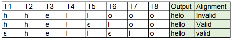
• In the first example since there is no ‘ϵ’ between the two ‘l’ we merge and predict a single ‘l’
• In the second example because of the presence of ‘ ϵ’ between the two ‘l’ we infer them as different.

2. Loss Calculation

To calculate the loss, we need to calculate the probability of generating the output sequence. Now since considering above there would be many valid alignments which could be reduced to generating the correct output. One naive approach would be to calculate all such valid alignments and sum over all the probabilities. However, this is computationally expensive and becomes impractical with an increase in input/output length.

Modified Sequence

To calculate CTC loss, we need to modify the input sequence to include blank symbols between each pair of characters. A modified Sequence​ is created by inserting blank symbols at the beginning and end of the original label sequence as well as between every pair of distinct non-blank labels.

Thus, an input word [‘ h e l l o’] is modified to [‘ϵ h ϵ e ϵ l ϵ l ϵ o ϵ’]

The purpose of introducing blanks is to allow for flexibility in aligning the input sequence with the output sequence without requiring a one-to-one correspondence between input and output symbols. How? This will become more intuitive once we see the forward-backward algorithm calculation below.
Each character in the modified sequence is known as state represented by (s). The CTC algorithm calculates two variables at each time stamp.

• Forward variable α(s, t): This variable represents the total probability of reaching state “s” at time “t”, having emitted the partial sequence up to that point.
• Backward variable β(s, t): This variable represents the total probability of emitting the remaining sequence from state “s” at time “t”.

This is the core of the CTC algorithm. This algorithm known as the forward-backward algorithm is used to calculate the loss. This forward-backward algorithm ‘calculates the probability of generating the required output at each step’. Let us see this mathematically.

Calculation of Forward Variable

To calculate the forward variable, we take the modified sequence and map it against the input time steps as shown in below diagram. Here we are assuming 11-time stamps of input audio.

Sample score calculation in CTC using DP

The model will output the probability of each token in the vocabulary y (s, t) at each time stamp. Now the problem that we need to solve is.

• Find valid states at each time sequence such that it leads to the predicted output. At each time stamp, only certain states will be valid to reach the expected output.
• For all such valid states calculate α(s, t) i.e. the probability of reaching the current valid state by considering all valid states that could be reached in the previous time stamp and which leads to a current valid state.

To solve the above we must follow below rules.

• Starting Prefixes with Blanks or First Symbol: We can either start with the special blank symbol or the correct prefix. This accommodates different alignment scenarios where the alignment may start with a blank or the first symbol of the label sequence.
• Allowing Transitions: At each time sequence we can do either of the below.
  • Transit between blank symbols and non-blank labels
  • Transit between any pair of distinct non-blank labels. Note we cannot transition between pairs of non-distinct symbols as we need to have a blank symbol in between ‘ε’
  • Remain in the state only.

The solution to the above problem is achieved through dynamic programming. As long as we know the values of all the valid α_{(s, t-1)} at the previous time-step, we can compute α_(s,t) at the current timestamp.

​Below is the algorithm:

• α_(0,0) = y_(0,0) and α_(1,0) = y_(1,0)
• for t = 0 to T-1:
  • for s = 0 to S
    • if s = ‘ε’ or s = s-2
      • 
    • else
      • 
• α_(s,t) = 0 for all s< S-2*(T-t)-1 correspond to states for which there are not enough time-steps left to complete the sequence (top right boxes)

Calculation of backward Variable

The backward variable represents the probability of observing the remaining part of the sequence from token s to the end of the sequence at timestep t. In other words, β_(s,t) computes the total probability of the subsequence Y_s:S​ given the current token s and timestep t.

The calculation of β(s,t) involves summing over all possible paths from the current position t to the end of the sequence while considering the transitions between different labels. The recursion formula for β(s,t) is as follows:

• β(s-1, t-1) = 1 and β(S-2, T-1) = 1
• for t = T-2 to 0:
  • for s = S-1 to 0
    • if s = ‘ε’ or s = s-2
      • 
    • else
      • 
• β(s,t) = 0 for all s< 2t which corresponds to the invalid states in the bottom-left

Total Probabilities

Using forward and backward variables we calculate the probability of getting the output sequence at a particular valid state as below.

γ(s, t) = α(s,t) * β(s,t) / y(s,t)

Here we need to divide by y(s,t) because it is getting included twice once in α(s, t) calculation and once in β(s,t) calculation.

This is done for all valid states at a particular time stamp. We then sum all the probabilities of all the valid states to get the total probability.

Loss can then be calculated as

Since the above formula involves multiplication and addition of probabilities derivatives can then be calculated for backpropagation.

3. Inference

Greedy Decoding:

After training the model, when selecting a likely output for a given input, a common heuristic involves choosing the most probable output at each time step. However, this approach may lead to inaccuracies in cases where the sum of probabilities for multiple alignments exceeds that of a single alignment. Consider the alignments [a, a, ϵ] and [a, a, a], each individually having a lower probability than [b, b, b]. Surprisingly, the combined probabilities of [a, a, a] and [a, a, ϵ] are greater than that of [b, b, b]. Using a naive heuristic might erroneously suggest that the most likely hypothesis is Y = [b], when, in fact, it should have been Y = [a]. To address this issue, the algorithm needs to account for the fact that [a, a, a] and [a, a, ϵ] collapse to the same output,

Beam Search:

A more sophisticated decoding approach is to use beam search. Beam search maintains a set of candidate sequences, or “beam,” and explores multiple possible paths through the output space. It keeps track of the most likely candidates at each step and prunes less likely paths to efficiently explore the search space.

• Initialize the beam with one or more candidate sequences. Each candidate sequence is associated with a score, which represents the log probability of the sequence given the input.
• For each candidate sequence in the current beam, extend it by considering the set of possible next tokens. In the context of CTC, this involves considering blank symbols and non-blank labels.
• Calculate the log probability score for each extended sequence based on the CTC probabilities.
• Choose the top candidates based on their scores, keeping the beam size in mind. Discard less likely candidates to maintain a manageable set.
• Select the sequence with the highest score from the final set of candidates as the decoded output sequence.

Applications of CTC

The CTC algorithm finds application in domains which do not require explicit alignment information between inputs and outputs during training like

1. Speech Recognition
2. Music Transcription
3. Gesture Recognition
4. In processing sensor data for robotics system

Advantages of CTC

1. CTC facilitates end-to-end training of neural networks for sequence-to-sequence tasks without the need for explicit alignment annotations.
2. It demonstrates resilience to labeling errors or inconsistencies within the training data by implicitly learning sequence alignments.
3. The algorithm is applicable across a diverse array of use cases, as outlined previously.

Challenges of CTC

1. The decoding phase in CTC can require significant computational resources, particularly when handling extended input sequences.
2. In speech recognition applications characterized by fluctuating acoustic environments, the CTC model may encounter challenges in effectively generalizing across diverse conditions.

IMPLEMENTATION OF CTC LOSS

In PyTorch, the ‘torch.nn.CTCLoss’ class is used to implement the Connectionist Temporal Classification (CTC) loss

Python3

import torch
import torch.nn as nn

ctc_loss = nn.CTCLoss()

loss = ctc_loss(log_probs, targets, input_lengths, target_lengths)

The arguments that needs to be passed are

• log_probs: The input sequence of log probabilities. It is typically the output of a neural network applied to the input sequence.
• targets: The target sequence. This is usually a 1-dimensional tensor of class indices.
• input_lengths: A 1-dimensional tensor containing the lengths of each sequence in the batch.
• target_lengths: A 1-dimensional tensor containing the lengths of each target sequence in the batch.

Assuming that we have a model, dataloader instantiated we can use CTC loss as below.

Python3

import torch
import torch.nn as nn
import torch.optim as optim

# First define your model

# Second define your dataloader to give inputs, targets,input_length and target_length


ctc_loss = nn.CTCLoss()
optimizer = optim.Adam(model.parameters(), lr=0.001)

for epoch in range(num_epochs):
    for inputs, targets, input_lengths, target_lengths in dataloader:
        optimizer.zero_grad()
        outputs = model(inputs)
        loss = ctc_loss(outputs, targets, input_lengths, target_lengths)
        loss.backward()
        optimizer.step()

One can adapt the above code as below:

• Define the neural network model for the sequence-to-sequence task.
• Ensure that the input and target sequences are appropriately shaped and padded. Define a DataLoader to iterate over your dataset, providing batches of input sequences (inputs), target sequences (targets), input sequence lengths (input_lengths), and target sequence lengths (target_lengths).
• Instantiate the CTC loss (nn.CTCLoss()) and an optimizer (Adam optimizer in this case) to optimize the parameters of your model.
• Intiate the training: The outer loop iterates over the specified number of epochs and the CTC loss is computed by comparing the predicted outputs (outputs) with the target sequences (targets).After calculating the loss, the gradients are computed via backpropagation (loss.backward()), and the optimizer is used to update the model parameters (optimizer.step()).

Conclusion

In this article, we saw how CTC loss can be used to train a neural network with different lengths of input and output. Its advantage lies in its ability to handle unaligned datasets during training, simplifying the training process significantly. The CTC algorithm can align variable-length input sequences with variable-length target sequences without the need for explicit alignment information during training.