While solving problems in real life it is very rare that we only come across binary classification problems because there are times when we have to classify within multiple categories for example dealing with the iris problem or the MNIST dataset is one of the common multiclass classification problems. As the researchers are developing the state of the art models they also keep this in mind to make the model work for multiclass classification problems.
Idea Behind using MultiClass Classification using LightGBM
As we know the lightGBM model is a light gradient-boosted machine that is used for the purpose of training on larger datasets in less time and getting decent results as well. As there are fewer models that support multiclass classification and the lightgbm model is one of them just we need to pass the right parameters to the model. We even do not have to convert it into the one hot encoded class it performs this on its own, which is an advantage here of using the LightGBM model for multi-class classification.
params = {
    'objective': 'multiclass',
    'num_class': 4,
    'metric': 'multi_logloss',
    'verbose': 0
}
For example in the above parameters:
- objective – We will set that to the multiclass which will tell teh model that we are trying to train a model on the multi-class classification dataset.
- metric – As the objective change we will have to change our metric as well we can use the multi_logloss, auc_mu or cross_entropy.
One more reason to use the LightGBM model is that it gives result comparative to the Neural Networks and as they are very efficient in tasks like this that is multi-class problems but implementing a NN for such a task can be tedious so, LightGBM comes handy and is easy to implement with some tweaks and twerks in the params of teh model.
Multiclass classification using LightGBM
In this article, we will learn about LightGBM model usage for the multiclass classification problem. This dataset has been used in this article to perform EDA on it and train the LightGBM model on this multiclass classification problem. But to use the LightGBM model we will first have to install the LightGBM model using the below command (in this article we are using version 3.3.5) :
!pip install lightgbm==3.3.5
Importing Libraries and Dataset
Python and its libraries are very helpful when given a large dataset which requires handling and processing.
- Pandas – This library is useful in loading the data and performing complex transformation.
- Numpy – Numpy arrays are useful when dealing with complex mathematical functions which require faster processing and performance
- Matplotlib/Seaborn – This library is useful in creating meaningful visualizations for better inference.
- Sklearn – This contains a vast library of useful functions which can be used for varied reasons like pre processing, predictions, etc.
Python3
import pandas as pd
import numpy as np
import seaborn as sb
import matplotlib.pyplot as plt
from sklearn.metrics import accuracy_score
from sklearn.preprocessing import StandardScaler
from sklearn.model_selection import train_test_split
import lightgbm as lgb
from sklearn.metrics import classification_report
import warnings
warnings.filterwarnings('ignore')
|
Now lets load the dataset into pandas dataframe.
Python3
df = pd.read_csv('bodyPerformance.csv')
df.head()
|
Output:
 age gender  height_cm  weight_kg  body fat_%  diastolic  systolic  \
0      27.0      M      172.3      75.24        21.3       80.0     130.0
1      25.0      M      165.0      55.80        15.7       77.0     126.0
2      31.0      M      179.6      78.00        20.1       92.0     152.0
3      32.0      M      174.5      71.10        18.4       76.0     147.0
4      28.0      M      173.8      67.70        17.1       70.0     127.0
...     ...    ...        ...        ...         ...        ...       ...
13388  25.0      M      172.1      71.80        16.2       74.0     141.0
13389  21.0      M      179.7      63.90        12.1       74.0     128.0
13390  39.0      M      177.2      80.50        20.1       78.0     132.0
13391  64.0      F      146.1      57.70        40.4       68.0     121.0
13392  34.0      M      164.0      66.10        19.5       82.0     150.0
       gripForce  sit and bend forward_cm  sit-ups counts  broad jump_cm class
0           54.9                     18.4            60.0          217.0     C
1           36.4                     16.3            53.0          229.0     A
2           44.8                     12.0            49.0          181.0     C
3           41.4                     15.2            53.0          219.0     B
4           43.5                     27.1            45.0          217.0     B
...          ...                      ...             ...            ...   ...
13388       35.8                     17.4            47.0          198.0     C
13389       33.0                      1.1            48.0          167.0     D
13390       63.5                     16.4            45.0          229.0     A
13391       19.3                      9.2             0.0           75.0     D
13392       35.9                      7.1            51.0          180.0     C
[13393 rows x 12 columns]
Output:
(13393, 12)
By using the df.info() function we can see the content of each columns and the data types present in it along with the number of null values present in each column.
Output:
<class 'pandas.core.frame.DataFrame'>
RangeIndex: 13393 entries, 0 to 13392
Data columns (total 12 columns):
 #   Column                   Non-Null Count  Dtype
---  ------                   --------------  -----
 0   age                      13393 non-null  float64
 1   gender                   13393 non-null  object
 2   height_cm                13393 non-null  float64
 3   weight_kg                13393 non-null  float64
 4   body fat_%               13393 non-null  float64
 5   diastolic                13393 non-null  float64
 6   systolic                 13393 non-null  float64
 7   gripForce                13393 non-null  float64
 8   sit and bend forward_cm  13393 non-null  float64
 9   sit-ups counts           13393 non-null  float64
 10  broad jump_cm            13393 non-null  float64
 11  class                    13393 non-null  object
dtypes: float64(10), object(2)
memory usage: 1.2+ MB
Descriptive statistical measures of the dataset help us better understand the data and it’s distribution over the plane. Let’s explore that to better understand it.
Output:
 age     height_cm     weight_kg    body fat_%     diastolic  \
count  13393.000000  13393.000000  13393.000000  13393.000000  13393.000000
mean      36.775106    168.559807     67.447316     23.240165     78.796842
std       13.625639      8.426583     11.949666      7.256844     10.742033
min       21.000000    125.000000     26.300000      3.000000      0.000000
25%       25.000000    162.400000     58.200000     18.000000     71.000000
50%       32.000000    169.200000     67.400000     22.800000     79.000000
75%       48.000000    174.800000     75.300000     28.000000     86.000000
max       64.000000    193.800000    138.100000     78.400000    156.200000
           systolic     gripForce  sit and bend forward_cm  sit-ups counts  \
count  13393.000000  13393.000000             13393.000000    13393.000000
mean     130.234817     36.963877                15.209268       39.771224
std       14.713954     10.624864                 8.456677       14.276698
min        0.000000      0.000000               -25.000000        0.000000
25%      120.000000     27.500000                10.900000       30.000000
50%      130.000000     37.900000                16.200000       41.000000
75%      141.000000     45.200000                20.700000       50.000000
max      201.000000     70.500000               213.000000       80.000000
       broad jump_cm
count   13393.000000
mean      190.129627
std        39.868000
min         0.000000
25%       162.000000
50%       193.000000
75%       221.000000
max       303.000000
Exploratory Data Analysis
Exploratory Data analysis (EDA), as the name suggests, is used to “explore” about the data. This means that in EDA, we are given with the task to learn about what story/pattern the dataset exhibits. This can be sued to get trends out of the dataset, find hidden patterns, check our hypothesis and much more, both in visual and statistical manner.
Python3
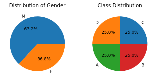
plt.subplot(1, 2, 1)
temp = df['gender'].value_counts()
plt.pie(temp.values, labels=temp.index.values,
autopct='%1.1f%%')
plt.title("Distribution of Gender")
plt.subplot(1, 2, 2)
temp = df['class'].value_counts()
plt.pie(temp.values, labels=temp.index.values,
autopct='%1.1f%%')
plt.title("Class Distribution")
plt.show()
|
Output:
In the dataset we can observe that the most of the columns are the numerical ones. And to explore the continuous data density plot is the most preferred one. But to create density plot iteratively we will have to first segregate all the numerical columns.
Python3
num_cols = list()
for col in df.columns:
if df[col].dtype == 'object':
continue
num_cols.append(col)
num_cols
|
Output:
['age',
 'height_cm',
 'weight_kg',
 'body fat_%',
 'diastolic',
 'systolic',
 'gripForce',
 'sit and bend forward_cm',
 'sit-ups counts',
 'broad jump_cm']
Now let’s create the density plot for all these numerical columns that we have segregated above.
Python3
plt.subplots(figsize=(8, 7))
for i, col in enumerate(num_cols):
plt.subplot(4, 3, i+1)
sb.distplot(df[col])
plt.tight_layout()
plt.show()
|
Output:
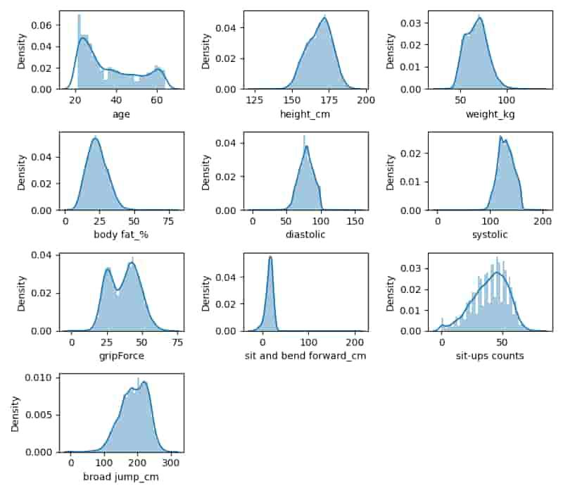
Distplot for various features
From the density plot above we can observe that the most of the numerical features are left skewed. And some of the features are normally distributed as well like BMI, Glucose, BloodPressure.
Python3
df['gender'] = df['gender'].map({'M': 0, 'F': 1})
df['class'] = df['class'].map({'A': 0, 'B': 1,
'C': 2, 'D': 3})
df.head()
|
Output:
age  gender  height_cm  weight_kg  body fat_%  diastolic  systolic  \
0      27.0       0      172.3      75.24        21.3       80.0     130.0
1      25.0       0      165.0      55.80        15.7       77.0     126.0
2      31.0       0      179.6      78.00        20.1       92.0     152.0
3      32.0       0      174.5      71.10        18.4       76.0     147.0
4      28.0       0      173.8      67.70        17.1       70.0     127.0
...     ...     ...        ...        ...         ...        ...       ...
13388  25.0       0      172.1      71.80        16.2       74.0     141.0
13389  21.0       0      179.7      63.90        12.1       74.0     128.0
13390  39.0       0      177.2      80.50        20.1       78.0     132.0
13391  64.0       1      146.1      57.70        40.4       68.0     121.0
13392  34.0       0      164.0      66.10        19.5       82.0     150.0
       gripForce  sit and bend forward_cm  sit-ups counts  broad jump_cm  \
0           54.9                     18.4            60.0          217.0
1           36.4                     16.3            53.0          229.0
2           44.8                     12.0            49.0          181.0
3           41.4                     15.2            53.0          219.0
4           43.5                     27.1            45.0          217.0
...          ...                      ...             ...            ...
13388       35.8                     17.4            47.0          198.0
13389       33.0                      1.1            48.0          167.0
13390       63.5                     16.4            45.0          229.0
13391       19.3                      9.2             0.0           75.0
13392       35.9                      7.1            51.0          180.0
       class
0          2
1          0
2          2
3          1
4          1
...      ...
13388      2
13389      3
13390      0
13391      3
13392      2
[13393 rows x 12 columns]
Finding Correlation between the features
Now we will find the correlation between the features in the dataset. It is to check that
Python3
sb.heatmap(df.corr(), annot=True,
cbar=True, cmap='RdBu', fmt='.1f')
plt.savefig('heatmap.png')
plt.show()
|
Output:
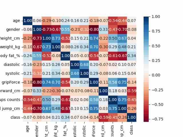
As there are no highly correlated feature (correlation greater than 0.8) in the dataset that can lead to data leakage or unnecessary increased complexity of the model, we can now move forward to data preprocessing and model development.
Model Development and Data Pre-processing
The first and the foremost step is that of splitting the data into training and the validation data. So, that we can monitor the training process of the model on some unforeseen data.
Python3
features = df.drop('class', axis=1)
target = df['class']
X_train, X_val,\
Y_train, Y_val = train_test_split(features, target,
random_state=2023,
test_size=0.20)
X_train.shape, X_val.shape
|
Output:
((10714, 11), (2679, 11))
Feature scaling proves to be very helpful in the fast and the stable training of the model.
Python3
scaler = StandardScaler()
scaler.fit(X_train)
X_train = scaler.transform(X_train)
X_val = scaler.transform(X_val)
|
Multiclass Classification using LightGBM
Before training an actual lightGBM model using the dataset first we will have to convert the dataset into lgb Datasets using lgb.Dataset API.
Python3
params = {
'objective': 'multiclass',
'num_class': 4,
'metric': 'multi_logloss',
'verbose': 0
}
train_data = lgb.Dataset(X_train, label=Y_train)
valid_data = lgb.Dataset(X_val, label=Y_val, reference=train_data)
|
Now as the parameters and the dataset has been defined let’s train the model.
Python3
num_round = 100
model = lgb.train(params,
train_data,
num_round,
early_stopping_rounds=10,
valid_sets=[valid_data])
|
Output:
[80]    valid_0's multi_logloss: 0.605381
[81]    valid_0's multi_logloss: 0.60547
[82]    valid_0's multi_logloss: 0.605018
[83]    valid_0's multi_logloss: 0.605324
[84]    valid_0's multi_logloss: 0.60554
[85]    valid_0's multi_logloss: 0.605153
[86]    valid_0's multi_logloss: 0.60477
Early stopping, best iteration is:
[76]    valid_0's multi_logloss: 0.604612
Now we can use the trained model to create predictions on the validation data.
Python3
y_pred = model.predict(X_val,
num_iteration=model.best_iteration)
y_pred.shape
y_pred[:4]
|
Output:
array([[8.77103321e-01, 9.94841889e-02, 2.05788684e-02, 2.83362177e-03],
       [1.19964248e-04, 1.08561258e-03, 1.06810300e-03, 9.97726320e-01],
       [2.04789377e-04, 1.22397780e-03, 2.83356414e-02, 9.70235591e-01],
       [6.00331842e-04, 2.70622699e-03, 9.55073045e-01, 4.16203966e-02]])
As we have got the probabilities for the four classes let’s use the argmax function to get the prediction classes.
Python3
y_pred = np.argmax(y_pred, axis=1)
y_pred[:10]
|
Output:
array([0, 3, 3, 2, 3, 0, 2, 3, 3, 2], dtype=int64)
Evaluation of the model
Now let’s evaluate the performance of the model using the validation data predictions.
Python3
accuracy = accuracy_score(Y_val, y_pred)
print(f'Accuracy: {accuracy}')
|
Output:
Accuracy: 0.7525195968645016
Let us check the classification report for the classes present in the dataset:
Python3
print(classification_report(Y_val, y_pred))
|
Output:
              precision    recall  f1-score   support
           0       0.74      0.88      0.80       661
           1       0.64      0.65      0.65       683
           2       0.73      0.66      0.69       642
           3       0.92      0.81      0.86       693
    accuracy                           0.75      2679
   macro avg       0.76      0.75      0.75      2679
weighted avg       0.76      0.75      0.75      2679
Conclusion
LightGBM can be considered to be a powerful and efficient tool for multiclass classification tasks. It can be useful when we are in need of faster computation and to handle large datasets. This algorithm can leverage it’s abilities to provide accurate predictions in a time crunched period.
Share your thoughts in the comments
Please Login to comment...