Binary classification using LightGBM

In this article, we will learn about one of the state-of-the-art machine learning models: Lightgbm or light gradient boosting machine. After improvising more and more on the XGB model for better performance XGBoost which is an eXtreme Gradient Boosting machine but by the lightgbm we can achieve similar or better results without much computing and train our model on an even bigger dataset in less time.

In this article, we will use this dataset to perform a classification task using the lightGBM algorithm. But to use the LightGBM model we will first have to install the lightGBM model using the below command:

Installing Packages

!pip install lightgbm

What is LightGBM and How it Works?

The “Light Gradient Boosting Machine,” an open-source, high-performance gradient boosting system, was developed for efficient and scalable machine learning applications. Because it is created expressly for speed and accuracy, it is a well-liked alternative for both organized and unstructured data in a range of areas. A few of LightGBM’s important characteristics include support for parallel and distributed processing, the ability to manage enormous datasets with millions of rows and columns, and better gradient-boosting techniques. LightGBM is known for its superior performance and little memory usage because of histogram-based techniques and leaf-wise tree growth.

An ensemble of decision trees is used by LightGBM, a powerful gradient-boosting framework renowned for its speed and precision. It begins with data that is arranged as instances and features and initializes a fundamental model with a wrong forecast. Following that, LightGBM establishes an objective function to calculate prediction errors and modifies model predictions using gradient data from this function. It is unique in that it builds trees according to the size of a leaf, choosing splits that minimize loss and producing deep, effective trees. It uses regularization techniques and early halting to stop overfitting. The efficiency of lightGBM is derived from histogram-based approaches, memory optimization, etc. The final forecast integrates contributions from individual trees.

Importing Libraries and Dataset

Python libraries make it very easy for us to handle the data and perform typical and complex tasks with a single line of code.

• Pandas – This library helps to load the data frame in a 2D array format and has multiple functions to perform analysis tasks in one go.
• Numpy – Numpy arrays are very fast and can perform large computations in a very short time.
• Matplotlib/Seaborn – This library is used to draw visualizations.
• Sklearn – This module contains multiple libraries having pre-implemented functions to perform tasks from data preprocessing to model development and evaluation.

Python3

import pandas as pd
import numpy as np
import seaborn as sb
import matplotlib.pyplot as plt
import lightgbm as lgb

from sklearn.preprocessing import StandardScaler
from sklearn.model_selection import train_test_split

import warnings
warnings.filterwarnings('ignore')

Loading Dataset and Retriving Information

Python3

df = pd.read_csv('Diabetes.csv')
df.head()

Output:

 Id  Pregnancies  Glucose  BloodPressure  SkinThickness  Insulin   BMI  \
0   1            6      148             72             35        0  33.6   
1   2            1       85             66             29        0  26.6   
2   3            8      183             64              0        0  23.3   
3   4            1       89             66             23       94  28.1   
4   5            0      137             40             35      168  43.1   
   DiabetesPedigreeFunction  Age  Outcome  
0                     0.627   50        1  
1                     0.351   31        0  
2                     0.672   32        1  
3                     0.167   21        0  
4                     2.288   33        1  

The dataset is being loaded at this time, and the top five rows are being printed.

Python3

df.shape

Output:

(2768, 10)

Here ‘df.shape’ prints the shape or the dimensions of the dataset.

Python3

df.info()

Output:

<class 'pandas.core.frame.DataFrame'>
RangeIndex: 2768 entries, 0 to 2767
Data columns (total 10 columns):
 #   Column                    Non-Null Count  Dtype  
---  ------                    --------------  -----  
 0   Id                        2768 non-null   int64  
 1   Pregnancies               2768 non-null   int64  
 2   Glucose                   2768 non-null   int64  
 3   BloodPressure             2768 non-null   int64  
 4   SkinThickness             2768 non-null   int64  
 5   Insulin                   2768 non-null   int64  
 6   BMI                       2768 non-null   float64
 7   DiabetesPedigreeFunction  2768 non-null   float64
 8   Age                       2768 non-null   int64  
 9   Outcome                   2768 non-null   int64  
dtypes: float64(2), int64(8)
memory usage: 216.4 KB

By using the df.info() function we can see the content of each columns and the data types present in it along with the number of null values present in each column.

Python3

df.describe()

Output:

               Id  Pregnancies      Glucose  BloodPressure  SkinThickness  \
count  2768.000000  2768.000000  2768.000000    2768.000000    2768.000000   
mean   1384.500000     3.742775   121.102601      69.134393      20.824422   
std     799.197097     3.323801    32.036508      19.231438      16.059596   
min       1.000000     0.000000     0.000000       0.000000       0.000000   
25%     692.750000     1.000000    99.000000      62.000000       0.000000   
50%    1384.500000     3.000000   117.000000      72.000000      23.000000   
75%    2076.250000     6.000000   141.000000      80.000000      32.000000   
max    2768.000000    17.000000   199.000000     122.000000     110.000000   
           Insulin          BMI  DiabetesPedigreeFunction          Age  \
count  2768.000000  2768.000000               2768.000000  2768.000000   
mean     80.127890    32.137392                  0.471193    33.132225   
std     112.301933     8.076127                  0.325669    11.777230   
min       0.000000     0.000000                  0.078000    21.000000   
25%       0.000000    27.300000                  0.244000    24.000000   
50%      37.000000    32.200000                  0.375000    29.000000   
75%     130.000000    36.625000                  0.624000    40.000000   
max     846.000000    80.600000                  2.420000    81.000000   
           Outcome  
count  2768.000000  
mean      0.343931  
std       0.475104  
min       0.000000  
25%       0.000000  
50%       0.000000  
75%       1.000000  
max       1.000000  

Descriptive statistical measures of the dataset help us better understand the data and it’s distribution over the plane. Here, the function ‘df.describe()’ computes and shows a basic statistical summary for the dataframe’s numeric columns.

Exploratory Data Analysis

EDA is an approach to analyzing the data using visual techniques. It is used to discover trends, and patterns, or to check assumptions with the help of statistical summaries and graphical representations. While performing the EDA of this dataset we will try to look at what is the relation between the independent features that is how one affects the other.

Visualizing Class Distribution

Python3

# Count the frequency of each class in the 'Outcome' column
temp = df['Outcome'].value_counts()

# Create a pie chart to represent class distribution
plt.pie(temp.values, labels=temp.index.values, autopct='%1.1f%%')

# Set the title of the chart
plt.title("Class Distribution")

# Display the pie chart
plt.show()

Output:

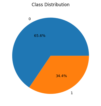
Here we can observe that the dataset at hand is not balanced for the two classes. We can use some data balancing techniques based on the target classes as well but this is not teh article for that purpose.

Visualizing Correlation Matrix Heatmap

Python3

# Compute the correlation matrix and create a heatmap with correlations above 0.7
sb.heatmap(df.corr() > 0.7, cbar=False, annot=True)

# Display the heatmap
plt.show()

Output:

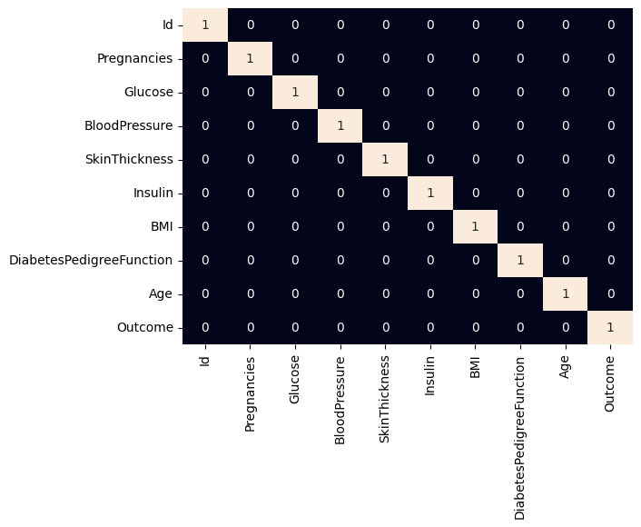
This code creates a heatmap using Seaborn to display a DataFrame’s correlation matrix. The color bar is hidden, while correlations greater than 0.7 are highlighted with annotated values. From the above correlation heatmap we can say that there are no highly correlated features. It is considered as a best practice to remove the highly correlated features from the feature set to avoid data leakage or the case of increased complexity of the program because of nothing.

Python3

# Create a count plot of 'Pregnancies' with 'Outcome' as the hue
sb.countplot(data=df, x='Pregnancies', hue='Outcome')

# Display the count plot
plt.show()

Output:

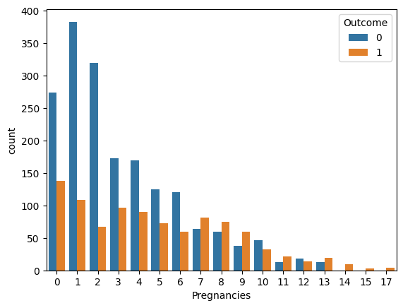
This code makes use of Seaborn to generate a count plot that shows the distribution of the ‘Pregnancies’ feature, with ‘Outcome’ acting as a colored indicator. It aids in tracking the distribution of pregnancies for various results. From the above countplot one of the interesting observation that we can make is that as the number of pregnancies increase the ratio of diabetes cases increases as well.

Visualizing Distributions of Features

Python3

# Create subplots to display distribution plots for each feature (excluding 'Id' and 'Outcome')
plt.subplots(figsize=(15, 15))

for i, col in enumerate(df.columns):
    if col in ['Id', 'Outcome']:
        continue
    plt.subplot(3, 3, i)
    sb.distplot(df[col])

# Adjust subplot layout for better presentation
plt.tight_layout()

# Display the distribution plots
plt.show()

Output:

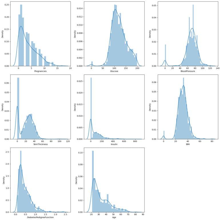
The numerical features in a DataFrame that are not “Id” and “Outcome” are generated by this code as a grid of distribution plots. Seaborn’s distplot tool is used to display the data distribution for each feature. Most of the features in the dataset are left skewed.

Data Preprocessing

To evaluate the performance of the model while the training process goes on let’s split the dataset in 80:20 ratio and then use it to create lgb dataset and then train the model.

Spliting Data

Python3

# Extracting features and target variable
features = df.drop('Outcome', axis=1)
target = df['Outcome']

# Splitting the data into training and validation sets with an 80-20 ratio
X_train, X_val, Y_train, Y_val = train_test_split(
    features, target, random_state=2023, test_size=0.20)

# Displaying the shapes of the training and validation sets
X_train.shape, X_val.shape

Output:

((2214, 9), (554, 9))

Feature scaling

Python3

# Initialize a StandardScaler
scaler = StandardScaler()

# Fit the scaler to the training data and transform both training and validation sets
scaler.fit(X_train)
X_train = scaler.transform(X_train)
X_val = scaler.transform(X_val)

Using StandardScaler from Scikit-Learn, this code applies standard scaling to the features. In order to ensure that the features have a mean of 0 and a standard deviation of 1, it calculates the mean and standard deviation from the training data and applies the same transformation to both the training and validation sets. This results in improved model performance.

Implementing Binary Classification using LightGBM

Let’s train the model on the training data and we will pass the validation data as well to visualize the performance of the model on the unseen data while training process goes on. This helps us to keep a check on the training progress.

Training a LightGBM Classifier

Python3

# Training a LightGBM Classifier
from lightgbm import LGBMClassifier

# Initialize a LightGBM Classifier with 'auc' as the evaluation metric
model = LGBMClassifier(metric='auc')

# Fit the model on the training data
model.fit(X_train, Y_train)

# Make predictions on the training and validation sets
y_train = model.predict(X_train)
y_val = model.predict(X_val)

The ‘auc‘ (Area Under the ROC Curve) metric is used as the evaluation metric in this code to train a LightGBM classifier. It then generates predictions for both the training and validation sets after fitting the model on the training set of data.

Creating LightGBM Dataset and Setting Parameters

Python3

# Creating LightGBM Dataset and Setting Parameters
import lightgbm as lgb

# Create LightGBM Datasets for training and validation
train_data = lgb.Dataset(X_train, label=Y_train)
test_data = lgb.Dataset(X_val, label=Y_val, reference=train_data)

# Define hyperparameters and objective for LightGBM
params = {
    'objective': 'binary',
    'metric': 'auc',
    'boosting_type': 'gbdt',
    'num_leaves': 31,
    'learning_rate': 0.05,
    'feature_fraction': 0.9,
}

Let’s take a quick look at the parameters that has been passed to the model.

• objective – This defines on what type of task you are going to train your model on for e.g binary has been passed here for binary classification task also we can pass regression and multi-class classification for regression ans multi class classification.
• metric – Metric that will be used by the model to improve upon. Also we will be able to get the model’s performance on the validation data(if passed) as the training process goes on.
• boosting_type – It is the method that is been used by the lightgbm model to train the parameters of the model for e.g GBDT(Gradient Boosting Decision Trees) that is the default method and rf(random forest based) and one more is dart(Dropouts meet Multiple Additive Regression Trees).
• num_leaves – The default value is 31 and it is used to define the maximum number of leaf nodes in a tree.
• learning_rate – As we know that the learning rate is a very common hyperparameter that is used to control the learning process.
• feature_fraction – This is the fraction of the features that will be used initially to train the decision trees. If we set this to 0.9 that means 90% of the features will be used only. this help us deal with the problem of overfitting.

Python3

# Training a LightGBM Model
num_round = 100

# Train a LightGBM model using defined parameters, training data, and specified number of rounds
model = lgb.train(params, train_data,
                  num_round, valid_sets=[test_data])

Output:

[90]    valid_0's auc: 0.994055
[91]    valid_0's auc: 0.994281
[92]    valid_0's auc: 0.99438
[93]    valid_0's auc: 0.994479
[94]    valid_0's auc: 0.994734
[95]    valid_0's auc: 0.995145
[96]    valid_0's auc: 0.995385
[97]    valid_0's auc: 0.995527
[98]    valid_0's auc: 0.995937
[99]    valid_0's auc: 0.996164
[100]    valid_0's auc: 0.996419

The parameters, training data, and predetermined number of training cycles (iterations) are used in this code to train a LightGBM model. During training, it verifies the model’s effectiveness using the test data.

Evaluation Of the Model

Now let’s check the performance of the model by using the ROC-AUC metric that is specifically used for evaluating the performance of a LightGBM model.

Python3

# Calculating and Printing ROC-AUC Scores
from sklearn.metrics import roc_auc_score as ras

# Calculate and print the ROC-AUC score for the training and validation sets
print("Training ROC-AUC: ", ras(Y_train, y_train))
print("Validation ROC-AUC: ", ras(Y_val, y_val))

Output:

Training ROC-AUC:  1.0
Validation ROC-AUC:  0.9946705357774791

This function generates the ROC-AUC values for the training and validation sets, giving an indication of the model’s performance in terms of categorization. From here we can say that the model is performing perfectly well on the training data also the ROC-AUC value for the validation data is also quite ideal.

Conclusion

Using LightGBM for binary classification, a variety of classification issues can be solved effectively and effectively. The main advantages of LightGBM are its capacity to handle big datasets with high-dimensional characteristics, which makes it a popular option in practical applications. LightGBM eases preprocessing chores and lessens the workload associated with data preparation because to its built-in procedures for categorical feature handling. The model’s robust feature importance analysis contributes to model interpretability by making it easier to grasp the variables influencing categorization choices. Classification accuracy can be accurately assessed by measuring model performance with metrics like ROC-AUC. To get the best results, however, extensive interpretability analysis and hyperparameter optimization are still crucial. In conclusion, LightGBM is a useful tool for binary classification jobs because it combines effectiveness, accuracy, and interpretability to effectively handle difficult machine learning challenges.