Perceptron Algorithm for Classification using Sklearn

Assigning a label or category to an input based on its features is the fundamental task of classification in machine learning. One of the earliest and most straightforward machine learning techniques for binary classification is the perceptron. It serves as the framework for more sophisticated neural networks. This post will examine how to use Scikit-Learn, a well-known Python machine-learning toolkit, to conduct binary classification using the Perceptron algorithm.

Perceptron

A simple binary linear classifier called a perceptron generates predictions based on the weighted average of the input data. Based on whether the weighted total exceeds a predetermined threshold, a threshold function determines whether to output a 0 or a 1. One of the earliest and most basic machine learning methods used for binary classification is the perceptron. Frank Rosenblatt created it in the late 1950s, and it is a key component of more intricate neural network topologies.

Single Layer Perceptron

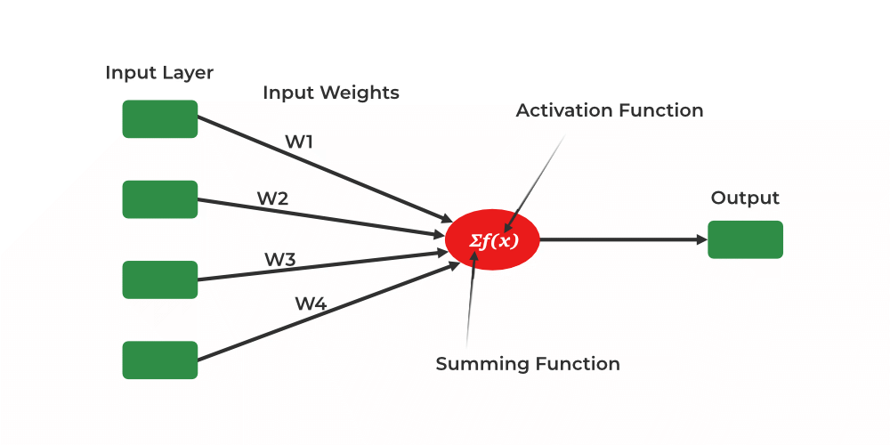
Components of a Perceptron:

1. Input Features (x): Predictions are based on the characteristics or qualities of the input data, or input features (x). A number value is used to represent each feature. The two classes in binary classification are commonly represented by the numbers 0 (negative class) and 1 (positive class).
2. Input Weights (w): Each input information has a weight (w), which establishes its significance when formulating predictions. The weights are numerical numbers as well and are either initialized to zeros or small random values.
3. Weighted Sum (): To calculate the weighted sum, use the dot product of the input features’ (x) weights and their associated features’ (w) weights. Mathematically, it is written as .
4. Activation Function (Step Function) : The activation function, which is commonly a step function, is applied to the weighted sum (). If the weighted total exceeds a predetermined threshold, the step function is utilized to decide the perceptron’s output. The output is 1 (positive class) if is greater than or equal to the threshold and 0 (negative class) otherwise.

Working of the Perceptron:

1. Initialization: The weights (w) are initially initialized, frequently using tiny random values or zeros.
2. Prediction: The Perceptron calculates the weighted total () of the input features and weights in order to provide a forecast for a particular input.
3. Activation Function: Following the computation of the weighted sum (), an activation function is used. The perceptron outputs 1 (positive class) if is greater than or equal to a specific threshold; otherwise, it outputs 0 (negative class) because the activation function is a step function.
4. Updating Weight: Weights are updated if a misclassification, or an inaccurate prediction, is made by the perceptron. The weight update is carried out to reduce prediction inaccuracy in the future. Typically, the update rule involves shifting the weights in a way that lowers the error. The perceptron learning rule, which is based on the discrepancy between the expected and actual class labels, is the most widely used rule.
5. Repeat: Each input data point in the training dataset is repeated through steps 2 through 4 one more time. This procedure keeps going until the model converges and accurately categorizes the training data, which could take a certain amount of iterations.

Sklearn (Scikit-Learn):

A strong Python framework for machine learning called Scikit-Learn offers straightforward and effective tools for modeling and data analysis. Use pip or conda to install scikit-learn if you already have a functioning installation of numpy and scipy.

pip install -U scikit-learn

conda install -c conda-forge scikit-learn

Steps required for classification using Perceptron:

There are various steps involved in performing classification using the Perceptron algorithm in Scikit-Learn:

1. Data preparation: Preprocess and load your dataset. A training set and a testing set should be separated.
2. Add Required Libraries: Import Scikit-Learn along with the other necessary libraries.
3. Perceptron Model Construction: Set hyperparameters like the learning rate and maximum iterations when creating a Perceptron classifier.
4. Training of the Model: Fit the training set of data to the perceptron model.
5. Make predictions: On the basis of the testing data, use the trained model to make predictions.
6. Model’s performance evaluation: Utilize metrics such as accuracy, precision, recall, and F1-score to evaluate the model’s performance.
7. Visualize the outcomes (optional): The decision boundary and the data points can be shown to help you see how the model categorizes cases.

Implementing Binary Classification using Perceptron

Let’s consider the few examples to understand the classification using Sklearn. In this example, we identify tumors as malignant or benign using the Breast Cancer Wisconsin dataset and a variety of characteristics, including mean radius, mean texture, and others.

Step 1: Importing necessary libraries

Python3

from sklearn.datasets import load_breast_cancer
from sklearn.linear_model import Perceptron
from sklearn.model_selection import train_test_split
from sklearn import metrics
from sklearn.metrics import accuracy_score
from sklearn.metrics import confusion_matrix

Step 2: Importing Breast Cancer Dataset

Using Scikit-Learn’s load_breast_cancer function, we load the Breast Cancer dataset. The features of breast cancer tumors are included in this dataset, along with the labels that correlate to them (0 for malignant and 1 for benign).

Python3

# Load the Breast Cancer dataset
data = load_breast_cancer()
X = data.data
y = data.target
print(X.shape)
print(y.shape)

Output:

(569, 30)
(569,)

Step3: Splitting the dataset in train and test set.

Python3

# Split the dataset into training and testing sets
X_train, X_test, y_train, y_test = train_test_split(X, y, test_size=0.3, random_state=42)
print(X_train.shape)
print(X_test.shape)
print(y_train.shape)
print(y_test.shape)

Output:

(398, 30)
(171, 30)
(398,)
(171,)

Step 4: Creating Perceptron

Python3

# Create a Perceptron model
clf = Perceptron(max_iter=1000, eta0=0.1)

Here max_iter defines the number of times the madel are used to train on the same dataset. and eta0 is the learning parameter.

Step 5 : Training the Perceptron Model

Using the Perceptron class from Scikit-Learn, we build a Perceptron model. We give the training’s maximum iteration count (max_iter) as well as the learning rate (eta0).

Python3

# Train the model
clf.fit(X_train, y_train)

Step 6: Prediction

For binary classification of tumour, we use the trained Perceptron model to make predictions on the testing data after training.

Python3

# Make predictions
y_pred = clf.predict(X_test)
print(y_pred)

Output:

[0 0 0 1 1 0 0 0 1 1 1 0 1 0 1 0 1 1 1 0 0 1 0 1 1 1 1 1 1 0 1 1 1 0 1 1 0
 1 0 1 1 0 1 1 1 1 1 1 1 1 0 0 1 1 1 1 1 0 1 1 1 0 0 1 1 1 0 0 1 1 0 0 1 1
 1 1 1 0 1 1 0 1 0 0 0 0 0 0 1 1 1 1 0 1 1 1 0 0 1 0 0 1 0 0 1 1 1 0 1 0 0
 1 1 0 1 0 1 1 1 0 0 1 1 0 1 0 0 1 1 0 0 1 0 1 0 0 1 1 0 0 1 0 1 1 0 1 0 0
 0 1 0 1 1 1 1 0 0 1 1 1 1 1 1 1 0 1 1 1 1 0 1]

Step 7: Evaluation

We assess the model’s accuracy in identifying malignant or benign tumors.

Python3

# Evaluate accuracy
accuracy = accuracy_score(y_test, y_pred)
print("Accuracy:", accuracy)

Output:

Accuracy: 0.935672514619883

Step 8: Confusion Matrix

Python3

# Calculate confusion matrix
conf_matrix = confusion_matrix(y_test, y_pred)
cm_display = metrics.ConfusionMatrixDisplay(confusion_matrix = conf_matrix, display_labels = [False, True])

cm_display.plot()
plt.show()

Output:

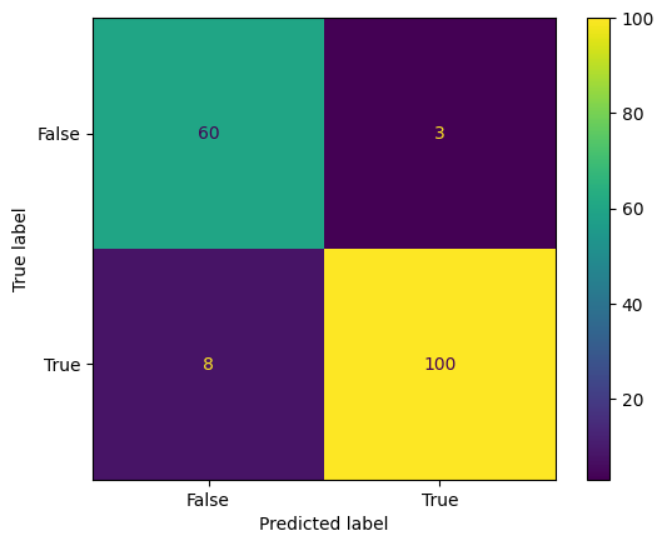
Heatmap of Confusion Matrix

Confusion Matrix shows the performance of the model where True negatives, false positives, false negatives, True positive values respectively.

Beyond Binary Classification:

While this article has mostly focused on binary classification, it is important to highlight that the Perceptron may also be extended to multiclass classification problems. It distributes instances to one of two classes in binary classification, but in multiclass classification, it may be altered to discriminate between several classes. This adaptation is frequently accomplished using tactics such as one-vs-all (OvA) or one-vs-one (OvO) strategies.

Implementing Multiclass Classification using Perceptron

In this example, our goal is to create a model based on pixel values that can identify handwritten digits (0-9) in text. The MNIST dataset is a well-known dataset for this job, which is a classic machine learning problem called handwritten digit recognition.

Step 1 : Importing necessary libraries

We start by loading the necessary libraries, including the MNIST dataset from sklearn.datasets and Scikit-Learn for machine learning operations.

Python3

from sklearn.datasets import fetch_openml
from sklearn.linear_model import Perceptron
from sklearn.model_selection import train_test_split
from sklearn.metrics import accuracy_score
import seaborn as sns

Step 2 : Loading dataset

Using the fetch_openml method from Scikit-Learn, we import the MNIST dataset. The MNIST dataset comprises of handwritten digits (0–9) and their related labels in 28×28 pixel pictures.

Python3

# Load the MNIST dataset
mnist = fetch_openml('mnist_784')
X = mnist.data
y = mnist.target.astype(int)
print(X.shape)
print(y.shape)

Output:

(70000, 784)
(70000,)

The dataset is loaded as a dictionary-like object in which the digit labels for each image’s pixels are located in mnist.target and its pixel values are stored in mnist.data.

Step 3: Splitting the Dataset into Test and Training set

Utilizing the train_test_split function of Scikit-Learn, we divided the dataset into training and testing sets. In this instance, 30% of the data are set aside for testing.

Python3

# Split the dataset into training and testing sets
X_train, X_test, y_train, y_test = train_test_split(X, y, test_size=0.3, random_state=42)

Step 4: Creating Perceptron Model

Using the Perceptron class from Scikit-Learn, we build a Perceptron model. We give the training’s maximum iteration count (max_iter) as well as the learning rate (eta0).

Python3

# Create a Perceptron model
perceptron = Perceptron(max_iter=1000, eta0=0.1)

Step 4: Model Training

Using the training set of data, we train the Perceptron model. Based on the pixel values of the images, the model develops the ability to differentiate between several digit classes.

Python3

# Train the model
perceptron.fit(X_train, y_train)

Step 5: Prediction

In order to forecast the digit labels for the test images, we use the trained Perceptron model to make predictions on the testing data after training.

Python3

# Make predictions
y_pred = perceptron.predict(X_test)
print(y_pred)

Output:

['8' '4' '8' ... '2' '9' '5']

Step 6: Evaluation

We determine the accuracy of the model’s predictions to evaluate its performance.

Python3

# Evaluate accuracy
accuracy = accuracy_score(y_test, y_pred)
print("Accuracy:", accuracy)

Output:

Accuracy: 0.87

Step 7: Confusion Matrix

Python3

# Calculate confusion matrix
conf_matrix = confusion_matrix(y_test, y_pred)

sns.heatmap(conf_matrix, annot = True, cmap= 'Blues')
plt.ylabel('True')
plt.xlabel('False')
plt.title('Confusion Matrix')
plt.show()

Output:

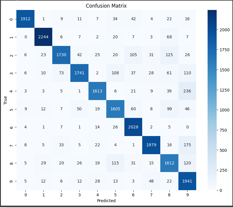
Heatmap for the Confusion Matrix

We calculate the confusion matrix using confusion_matrix(y_test, y_pred), where y_test contains the true labels, and y_pred contains the predicted labels. We use matplotlib and seaborn to create a heatmap visualization of the confusion matrix, making it easier to interpret. The heatmap is annotated with the actual numerical values from the confusion matrix. The x-axis represents the predicted labels, and the y-axis represents the true labels.

Challenges and Limitations

One of the main disadvantages of using perceptron is that it cannot handle non-linearly separable data. This means that the Perceptron will struggle to produce accurate predictions if your data cannot be neatly separated into two groups using a straight line (or hyperplane in higher dimensions). More advanced methods, such as support vector machines (SVMs) and deep neural networks, have been created to alleviate this shortcoming.

Modern deep learning frameworks and architectures, such as convolutional neural networks (CNNs) and recurrent neural networks (RNNs), have far outperformed the Perceptron in terms of performance and adaptability.

Understanding the Perceptron, on the other hand, is essential for laying a firm basis in machine learning. It explains the fundamental concepts of categorization as well as the idea of linear decision limits. As you proceed through your machine learning adventure, you’ll realize the Perceptron’s historical relevance and role in defining the area of artificial intelligence.

Conclusion

In this article, we have used the Perceptron, a flexible and popular machine learning framework in Python for classification. We also had discussed instances demonstrating the Perceptron’s efficiency in resolving various categorization problems. Perceptron is a fundamental building element in the development of machine learning, despite being relatively simple in comparison to more complex algorithms. It offers insightful information on the principles underlying linear decision boundaries and binary classification. It’s important to note that more sophisticated approaches like deep neural networks, support vector machines, or ensemble methods are frequently used for complex and high-dimensional data.