Anomaly Detection Using R

Anomaly detection is a critical aspect of data analysis, allowing us to identify unusual patterns, outliers, or abnormalities within datasets. It plays a pivotal role across various domains such as finance, cybersecurity, healthcare, and more.

What is Anomalies?

Anomalies, also known as outliers, are data points that significantly deviate from the normal behavior or expected patterns within a dataset. They can be caused by various factors such as errors in data collection, system glitches, fraudulent activities, or genuine but rare occurrences.

Detecting anomalies in R Programming Language involves distinguishing between normal and abnormal behaviors within the data. This process is crucial for decision-making, risk management, and maintaining the integrity of datasets. They can manifest in various forms and fields.

1. Financial Transactions

In financial data, anomalies might include fraudulent activities like:

• Unusually large transactions compared to typical spending patterns for an individual.
• Transactions occurring at odd hours or from atypical geographic locations.
• in spending behavior.

2. Network Security

In cybersecurity, anomalies could be:

• Unusual spikes in network traffic that differ significantly from regular patterns.
• Unexpected login attempts from unrecognized IP addresses.
• Unusual file access or transfer patterns that deviate from typical user behavior.

3. Healthcare and Medical Data

In medical data, anomalies might include:

• Outliers in patient vital signs that deviate significantly from the norm.
• Irregularities in medical imaging (like X-rays, MRIs) indicating potential health issues.
• Unexpected patterns in patient records, such as sudden, significant changes in medication or treatment adherence.

4. Manufacturing and IoT

In manufacturing or IoT (Internet of Things), anomalies could be:

• Abnormal sensor readings in machinery indicating potential faults or malfunctions.
• Sudden temperature, pressure, or vibration changes in equipment beyond usual operating ranges.
• Deviations in product quality or output that fall outside standard tolerances.

5. Climate and Environmental Data

In environmental datasets, anomalies might be:

• Unusual weather patterns or extreme weather events that deviate from historical records.
• Unexpected changes in air quality measurements indicating potential pollution events.
• Abnormal fluctuations in ocean temperatures or ice melting rates.

Identifying anomalies in these scenarios can be crucial for fraud detection, system monitoring, predictive maintenance, healthcare diagnosis, and decision-making across various industries. Detection methods and techniques like statistical analysis, machine learning algorithms, or domain-specific rules are applied to uncover and address anomalies in datasets for better insights and informed actions.

Types of Anamolies

Global Outliers

These are individual data points that deviate significantly from the overall pattern in the entire dataset.

Consider a dataset representing the average income of residents in a city. Most people in the city have incomes between $30,000 and $80,000 per year. However, there is one individual in the dataset with an income of $1 million. This individual’s income is significantly higher than the overall pattern of incomes in the entire dataset, making it a global outlier.

Contextual Outliers:

Anomalies that are context-specific. They may not be considered outliers when looking at the entire dataset, but they stand out in a particular subset or context.

Imagine you are analyzing the sales performance of products in different regions. In the overall dataset, a particular product might have average sales. However, when you focus on a specific region, you notice that the sales for that product are exceptionally low compared to other products in that region. In this context (specific region), the low sales for that product make it a contextual outlier.

Collective Outliers (or Collective Anomalies)

Anomalies that involve a group of data points or a pattern of behavior that is unusual when considered as a whole, rather than focusing on individual data points.

Suppose you are monitoring the network traffic in a computer system. Individually, certain data packets may not be considered outliers, but when analyzed collectively, a sudden surge in traffic from multiple sources is detected. This unusual pattern of behavior, involving a group of data points (data packets), is considered a collective outlier because the overall behavior of the system as a whole deviates from the expected pattern.

Visualization of Anamolies

Now we will plot the Anamolies for a better understanding of the users.

Scatter Plot

R

# Install and load the ggplot2 package
install.packages("ggplot2")
library(ggplot2)

# Sample dataset with two numeric features and an indicator for anomalies
set.seed(123)
data <- data.frame(
  Feature1 = rnorm(100),
  Feature2 = rnorm(100),
  is_anomaly = rep(c(0, 1), each = 50)  # Assuming half of the data is anomalous
)

# Scatter plot with anomalies marked in red
ggplot(data, aes(x = Feature1, y = Feature2, color = factor(is_anomaly))) +
  geom_point() +
  scale_color_manual(values = c("0" = "blue", "1" = "red")) +
  labs(title = "Scatter Plot with Anomalies Highlighted",
       x = "Feature 1", y = "Feature 2",
       color = "Anomaly") +
  theme_minimal()

Output:

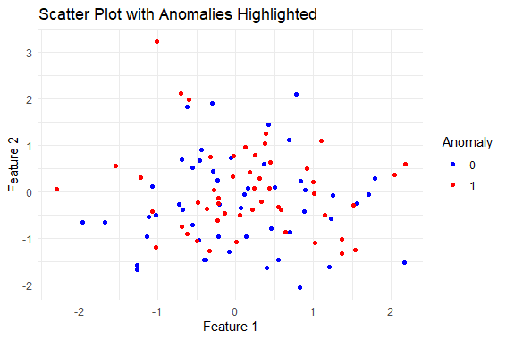
Anomaly Detection Using R

Line chart

R

# Install and load the ggplot2 package
install.packages("ggplot2")
library(ggplot2)

# Sample dataset with a numeric variable and an indicator for anomalies
set.seed(123)
data <- data.frame(
  Time = 1:50,
  Value = c(rnorm(25), rnorm(25, mean = 5)),
  is_anomaly = c(rep(0, 25), rep(1, 25))
)

# Line chart with anomalies emphasized
ggplot(data, aes(x = Time, y = Value, color = factor(is_anomaly))) +
  geom_line() +
  geom_point(data = subset(data, is_anomaly == 1), color = "red", size = 3) +
  scale_color_manual(values = c("0" = "blue", "1" = "red")) +
  labs(title = "Line Chart with Anomalies Emphasized",
       x = "Time", y = "Value",
       color = "Anomaly") +
  theme_minimal()

Output:

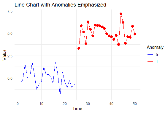
Anomaly Detection Using R

Anomaly Detection Techniques in R

Statistical Methods

WE have several methods in Statistical Methods for Anomaly Detection Using R.

Z-Score

The Z-score measures the deviation of a data point from the mean in terms of standard deviations. In R, the `scale()` function is often used to compute Z-scores, and points beyond a certain threshold (typically 2 or 3 standard deviations) are considered anomalies.

The Z-score is a statistical measurement that quantifies how far a data point is from the mean of a dataset in terms of standard deviations. It’s calculated using the formula:

Z = X-μ / σ

Where:

• X is the individual data point.
• μ is the mean of the dataset.
• σ is the standard deviation of the dataset.

Let’s Implement Z Score in R

R

# Sample exam scores
scores <- c(75, 82, 90, 68, 88, 94, 78, 60, 72, 85)

# Calculate mean and standard deviation
mean_score <- mean(scores)
std_dev <- sd(scores)

# Calculate Z-scores for each data point
z_scores <- (scores - mean_score) / std_dev

# Display the Z-scores
z_scores

Output:

 [1] -0.3945987  0.2630658  1.0146823 -1.0522632  0.8267782  1.3904906 -0.1127425
 [8] -1.8038797 -0.6764549  0.5449220

For this example dataset

• Mean (μ) = 79.2
• Standard deviation (σ) ≈ 10.59

The Z-scores would be calculated for each data point using the formula. These scores represent how many standard deviations each data point is away from the mean.

Grubbs’ Test

This test identifies outliers in a univariate dataset by iteratively removing the most extreme value until no more outliers are found. The `outliers` package in R provides functions like `grubbs.test()` for this purpose.

Let’s Implement this in R.

R

# Install and load the outliers package
# install.packages("outliers")
library(outliers)

# Example dataset with outliers
data_with_outliers <- c(10, 12, 15, 20, 22, 25, 30, 35, 50, 300, 22, 18, 13, 11, 10)

# Perform Grubbs' Test to detect outliers
outlier_test <- grubbs.test(data_with_outliers)

# Display the test results
outlier_test

Output:

    Grubbs test for one outlier
data:  data_with_outliers
G = 3.573988, U = 0.022445, p-value = 3.149e-11
alternative hypothesis: highest value 300 is an outlier

In this example

• The data_with_outliers vector contains a set of numbers, including outliers such as 300.
• grubbs.test() analyzes the dataset and performs Grubbs’ Test to identify potential outliers.
• The test result will display the Grubbs’ test statistic and the critical value, indicating if any outliers were detected in the dataset.

2. Density Based Anamoly Detection

• Density-based methods identify anomalies based on the local density of data points. Outliers are often located in regions with lower data density.
• The dbscan package in R is commonly used for density-based clustering, which can be adapted for anomaly detection.

R

# Install and load the dbscan package
#install.packages("dbscan")
library(dbscan)

# Generate some example data
set.seed(123)
data <- matrix(rnorm(200), ncol = 2)

# Implement density-based clustering for anomaly detection
result <- dbscan(data, eps = 0.5, minPts = 5)

# Print the clustering result
print(result)

# Identify noise points (potential anomalies)
anomalies <- which(result$cluster == 0)

# Print the indices of potential anomalies
print(anomalies)

Output:

DBSCAN clustering for 100 objects.
Parameters: eps = 0.5, minPts = 5
Using euclidean distances and borderpoints = TRUE
The clustering contains 1 cluster(s) and 20 noise points.
 0  1 
20 80 
Available fields: cluster, eps, minPts, dist, borderPoints
 [1]  8 13 18 21 25 26 35 37 39 43 44 49 57 64 70 72 74 78 96 97

3. Cluster-Based Anomaly Detection

• Cluster-based methods involve grouping similar data points into clusters and identifying anomalies as data points that do not belong to any cluster or belong to small clusters.
• The kmeans function in base R or the cluster package can be used for cluster-based anomaly detection.

R

# Generate some example data
set.seed(123)
data <- matrix(rnorm(200), ncol = 2)

# Perform k-means clustering
kmeans_result <- kmeans(data, centers = 3)

# Print the clustering result
print(kmeans_result)

# Identify anomalies based on cluster membership
anomalies <- which(kmeans_result$cluster == 1)

# Print the indices of potential anomalies
print(anomalies)

Output:

K-means clustering with 3 clusters of sizes 38, 29, 33
Cluster means:
         [,1]       [,2]
1 -0.66333772 -0.6219885
2 -0.02025692  1.0093022
3  1.05560227 -0.4966328
Clustering vector:
  [1] 1 2 3 1 1 3 3 1 1 2 3 2 3 1 2 3 3 1 3 1 1 1 1 1 2 1 3 2 1 3 2 2 3 3 3 2 3 2 2 1
 [41] 2 1 1 3 3 1 1 2 2 1 2 2 2 3 1 3 1 3 2 3 2 1 1 2 1 2 2 1 3 3 1 1 3 2 1 3 1 1 2 1
 [81] 1 2 1 3 1 3 2 3 2 3 3 3 2 1 3 2 3 3 1 1
Within cluster sum of squares by cluster:
[1] 23.92627 22.26036 24.96196
 (between_SS / total_SS =  59.4 %)
Available components:
[1] "cluster"      "centers"      "totss"        "withinss"     "tot.withinss"
[6] "betweenss"    "size"         "iter"         "ifault"      
 [1]   1   4   5   8   9  14  18  20  21  22  23  24  26  29  40  42  43  46  47  50
[21]  55  57  62  63  65  68  71  72  75  77  78  80  81  83  85  94  99 100

4. Bayesian Network Anomaly Detection

• Bayesian networks model the probabilistic relationships between variables. Anomalies can be detected by identifying instances where observed data significantly deviates from the expected probabilities.
• The bnlearn package is commonly used for Bayesian network modeling.

R

# Load the package
install.packages("bnlearn")
library(bnlearn)

# Generate some example data
set.seed(123)
data <- data.frame(
  A = rnorm(100),
  B = rnorm(100),
  C = rnorm(100)
)

# Define the structure of the Bayesian network
# For example, A and B are parents of C
network_structure <- model2network("[A][B][C|A:B]")

# Build a Bayesian network
bn_model <- bn.fit(network_structure, data)
print(bn_model)

Output:

  Bayesian network parameters
  Parameters of node A (Gaussian distribution)
Conditional density: A
Coefficients:
(Intercept)  
 0.09040591  
Standard deviation of the residuals: 0.9128159 
  Parameters of node B (Gaussian distribution)
Conditional density: B
Coefficients:
(Intercept)  
 -0.1075468  
Standard deviation of the residuals: 0.9669866 
  Parameters of node C (Gaussian distribution)
Conditional density: C | A + B
Coefficients:
(Intercept)            A            B  
 0.13506543  -0.13317153   0.02381129  
Standard deviation of the residuals: 0.9512979 

5.Autoencoders

Autoencoders are a type of neural network used for unsupervised learning that aims to reconstruct input data. Anomalies may result in higher reconstruction errors compared to normal instances. e.g: Imagine trying to redraw something from memory; mistakes might signal something unusual.

R

# Load necessary libraries
library(keras)

# Generate sample data
set.seed(123)
normal_data <- as.matrix(data.frame(x = rnorm(1000), y = rnorm(1000)))
anomalies <- as.matrix(data.frame(x = runif(10, 5, 10), y = runif(10, -10, -5)))
data <- rbind(normal_data, anomalies)

# Build autoencoder model
model <- keras_model_sequential() %>%
  layer_dense(units = 8, activation = 'relu', input_shape = ncol(data)) %>%
  layer_dense(units = 2, activation = 'relu') %>%
  layer_dense(units = 8, activation = 'relu') %>%
  layer_dense(units = ncol(data))

# Compile the model
model %>% compile(optimizer = 'adam', loss = 'mse')

# Fit the model
history <- model %>% fit(data, data, epochs = 50, batch_size = 32,
                         validation_split = 0.2, verbose = 0)

# Reconstruct data
reconstructed_data <- model %>% predict(data)
reconstruction_error <- rowMeans((data - reconstructed_data)^2)

# Visualize anomalies (scatter plot with heading)
plot(data, col = ifelse(reconstruction_error > quantile(reconstruction_error, 0.95),
                        "red", "blue"), pch = 19,
     main = "Autoencoder Anomaly Detection", xlab = "X-axis", ylab = "Y-axis")
legend("topright", legend = c("Normal", "Anomaly"), col = c("blue", "red"), pch = 19)

Output:

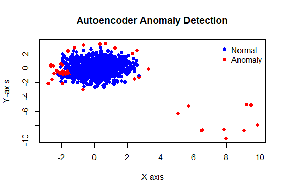
Anomaly Detection Using R

Difference Between Different Techniques

Technique	Method	Key Features	Applicability
Statistical Methods	Z-Score, Grubbs’ Test	Measures deviation from mean in standard deviations.	General datasets, univariate data
Density-Based	DBSCAN	Identifies anomalies based on local density.	Suitable for various domains
Cluster-Based	K-Means	Groups similar data points into clusters.	Applicable to diverse datasets
Bayesian Network	bnlearn	Models probabilistic relationships between variables.	Effective for interconnected data
One-Class SVM (OCSVM)	SVM	Learns a boundary around normal data instances.	Effective for known normal patterns
Autoencoders	Neural Network	Used for unsupervised learning, detects anomalies via reconstruction errors.	Suitable for complex patterns

Challenges in Anomaly Detection

1. Imbalanced Data: Anomalies are rare compared to normal data, leading to imbalanced datasets and biased models.
2. False Positives/Negatives: Balancing accurate anomaly detection without raising too many false alarms or missing actual anomalies remains a challenge.
3. Interpretability: Complex models often lack interpretability, making it hard to understand why an instance is flagged as an anomaly.
4. Scalability: Implementing anomaly detection on large datasets or real-time streams can be computationally expensive.
5. Data Quality: Distinguishing between genuine anomalies and data errors is difficult, affecting detection reliability.
6. Adaptability: Models might struggle with evolving patterns or unseen anomalies, impacting their effectiveness.
7. Threshold Selection: Setting appropriate thresholds for anomaly detection across diverse data patterns is challenging and requires constant adjustments.

Advantages of Anomaly Detection

1. Early Problem Spotting: Helps find issues before they become big problems.
2. Risk Reduction: Lowers risks by spotting abnormal behavior early.
3. Better Decision-Making: Gives insights for smarter decisions based on accurate data.
4. Enhanced Security: Crucial for cybersecurity by spotting intrusions or unusual network activity.
5. Predictive Maintenance: Helps prevent equipment breakdowns by finding faults early.
6. Healthcare Help: Identifies health issues sooner by spotting unusual signs.
7. Efficiency Boost: Improves efficiency by finding things affecting productivity.

Disadvantages of Anomaly Detection

1. False Alarms: Sometimes flags normal things as problems or misses real issues.
2. Complex Understanding: Some methods are hard to understand.
3. High Computing Needs: Certain techniques need lots of computer power and time.
4. Adapting to Changes: Struggles to spot new issues without extra training.
5. Threshold Challenges: Setting the right detection levels for different situations can be tough.
6. Data Imbalance: Rare anomalies can make the data uneven, leading to bias.
7. Data Quality Issues: Hard to tell if something’s an anomaly or just a data mistake.

Future Scope of Anamoly Detection

1. Deep Learning Integration: Expect deeper integration of neural networks for better pattern recognition.
2. Unsupervised Learning Advances: Algorithms improving without labeled data for adaptability.
3. Explainable AI (XAI) Emphasis: Focus on transparent anomaly detection models.
4. Edge Computing Applications: Real-time detection in distributed systems.
5. AutoML and Model Optimization: Streamlined selection and optimization.
6. Adversarial Anomaly Detection: Detection improvement against evasive anomalies.
7. Hybrid Multimodal Approaches: Integrating diverse data types for comprehensive analysis.

Conclusion

Anomaly detection is a key part of data analysis. It helps find odd things in data from different industries. Using R’s strong tools, experts can find and handle these odd things well. Mastering these methods helps organizations not only find oddities but also prevent problems, make smart choices with data, and keep data reliable. This important role of anomaly detection is crucial for smart choices, staying safe, and keeping data trustworthy in different areas.