RNN for Text Classifications in NLP

In this article, we will learn how we can use recurrent neural networks (RNNs) for text classification tasks in natural language processing (NLP). We would be performing sentiment analysis, one of the text classification techniques on the IMDB movie review dataset. We would implement the network from scratch and train it to identify if the review is positive or negative.

RNN for Text Classifications in NLP

In Natural Language Processing (NLP), Recurrent Neural Networks (RNNs) are a potent family of artificial neural networks that are crucial, especially for text classification tasks. RNNs are uniquely able to capture sequential dependencies in data, which sets them apart from standard feedforward networks and makes them ideal for processing and comprehending sequential information, like language. RNNs are particularly good at evaluating the contextual links between words in NLP text classification, which helps them identify patterns and semantics that are essential for correctly classifying textual information. Because of their versatility, RNNs are essential for creating complex models for tasks like document classification, spam detection, and sentiment analysis.

Recurrent Neural Networks (RNNs)

Recurrent neural networks are a specific kind of artificial neural network created to work with sequential data. It is utilized particularly in activities involving natural language processing, such as language translation, speech recognition, sentiment analysis, natural language generation, and summary writing. Unlike feedforward neural networks, RNNs include a loop or cycle built into their architecture that acts as a “memory” to hold onto information over time. This distinguishes them from feedforward neural networks.

Implementation of RNN for Text Classifications

First, we will need the following dependencies to be imported.

Python3

import tensorflow as tf
import tensorflow_datasets as tfds

import numpy as np
import matplotlib.pyplot as plt

The code imports the TensorFlow library (tf) along with its dataset module (tensorflow_datasets as tfds). Additionally, it imports NumPy (np) for numerical operations and Matplotlib (plt) for plotting. These libraries are commonly used for machine learning tasks and data visualization.

1. Load the dataset

IMDB movies review dataset is the dataset for binary sentiment classification containing 25,000 highly polar movie reviews for training, and 25,000 for testing. This dataset can be acquired from this website or we can also use tensorflow_datasets library to acquire it.

Python3

# Obtain the imdb review dataset from tensorflow datasets
dataset = tfds.load('imdb_reviews', as_supervised=True)

# Seperate test and train datasets
train_dataset, test_dataset = dataset['train'], dataset['test']

# Split the test and train data into batches of 32
# and shuffling the training set
batch_size = 32
train_dataset = train_dataset.shuffle(10000)
train_dataset = train_dataset.batch(batch_size)
test_dataset = test_dataset.batch(batch_size)

The code loads the IMDb review dataset using TensorFlow Datasets (tfds.load(‘imdb_reviews’, as_supervised=True)). It then separates the dataset into training and testing sets (train_dataset and test_dataset). Finally, it batches the training and testing data into sets of 32 samples each, and shuffles the training set to enhance the learning process by preventing the model from memorizing the order of the training samples. The batch_size variable determines the size of each batch.

Printing a sample review and its label from the training set.

Python3

example, label = next(iter(train_dataset))
print('Text:\n', example.numpy()[0])
print('\nLabel: ', label.numpy()[0])

Output:

Text:
 b'Stumbling upon this HBO special late one night, I was absolutely taken by this 
 attractive British "executive transvestite." I have never laughed so hard over 
 European History or any of the other completely worthwhile point Eddie Izzard made.
  I laughed so much that I woke up my mother sleeping at the other end of the house...'
Label:  1

The code uses the iter function to create an iterator for the training dataset and then extracts the first batch using next(iter(train_dataset)). It prints the text of the first example in the batch (example.numpy()[0]) and its corresponding label (label.numpy()[0]). This provides a glimpse into the format of the training data, helping to understand how the text and labels are structured in the IMDb review dataset.

2. Build the Model

In this section, we will define the model we will use for sentiment analysis. The initial layer of this architecture is the text vectorization layer, responsible for encoding the input text into a sequence of token indices. These tokens are subsequently fed into the embedding layer, where each word is assigned a trainable vector. After enough training, these vectors tend to adjust themselves such that words with similar meanings have similar vectors. This data is then passed to RNN layers which process these sequences and finally convert it to a single logit as the classification output.

Text Vectorization

We will first perform text vectorization and let the encoder map all the words in the training dataset to a token. We can also see in the example below how we can encode and decode the sample review into a vector of integers.

Python3

# Using the TextVectorization layer to normalize, split, and map strings
# to integers.
encoder = tf.keras.layers.TextVectorization(max_tokens=10000)
encoder.adapt(train_dataset.map(lambda text, _: text))

# Extracting the vocabulary from the TextVectorization layer.
vocabulary = np.array(encoder.get_vocabulary())

# Encoding a test example and decoding it back.
original_text = example.numpy()[0]
encoded_text = encoder(original_text).numpy()
decoded_text = ' '.join(vocabulary[encoded_text])

print('original: ', original_text)
print('encoded: ', encoded_text)
print('decoded: ', decoded_text)

Output:

original: 
 b'Stumbling upon this HBO special late one night, I was absolutely taken by this 
 attractive British "executive transvestite." I have never laughed so hard over 
 European History or any of the other completely worthwhile point Eddie Izzard made. 
 I laughed so much that I woke up my mother sleeping at the other end of the house...'
encoded: 
 [9085  720   11 4335  309  534   29  311   10   14  412  602   33   11
 1523  683 3505    1   10   26  110 1434   38  264  126 1835  489   42
   99    5    2   81  325 2601  215 1781 9352   91   10 1434   38   73
   12   10 9259   58   56  462 2703   31    2   81  129    5    2  313]
decoded: 
 stumbling upon this hbo special late one night i was absolutely taken by this 
 attractive british executive [UNK] i have never laughed so hard over european history
  or any of the other completely worthwhile point eddie izzard made i laughed so much 
  that i woke up my mother sleeping at the other end of the house

The code defines a TextVectorization layer (encoder) with a vocabulary size limit of 10,000 tokens and adapts it to the training dataset. It then extracts the vocabulary from the TextVectorization layer. The code encodes an example text using the TextVectorization layer (encoder(original_text).numpy()) and decodes it back to the original form using the vocabulary. This demonstrates how the TextVectorization layer can normalize, tokenize, and map strings to integers, facilitating text processing for machine learning models.

Create the model

Now, we will use this trained encoder along with other layers to define a model as discussed earlier. In TensorFlow, while the RNN layers cannot be directly used with a Bidirectional wrapper and Embedding layer, we can employ its derivatives, like LSTM (Long Short-Term Memory) and GRU (Gated Recurrent Unit). In this example, we will use LSTM layers to define the model.

Python3

# Creating the model
model = tf.keras.Sequential([
    encoder,
    tf.keras.layers.Embedding(
        len(encoder.get_vocabulary()), 64, mask_zero=True),
    tf.keras.layers.Bidirectional(
        tf.keras.layers.LSTM(64,  return_sequences=True)),
    tf.keras.layers.Bidirectional(tf.keras.layers.LSTM(32)),
    tf.keras.layers.Dense(64, activation='relu'),
    tf.keras.layers.Dense(1)
])

# Summary of the model
model.summary()

# Compile the model
model.compile(
    loss=tf.keras.losses.BinaryCrossentropy(from_logits=True),
    optimizer=tf.keras.optimizers.Adam(),
    metrics=['accuracy']
)

Output:

Model: "sequential"
_________________________________________________________________
 Layer (type)                Output Shape              Param #   
=================================================================
 text_vectorization (TextVe  (None, None)              0         
 ctorization)                                                    
                                                                 
 embedding (Embedding)       (None, None, 64)          640000    
                                                                 
 bidirectional (Bidirection  (None, None, 128)         66048     
 al)                                                             
                                                                 
 bidirectional_1 (Bidirecti  (None, 64)                41216     
 onal)                                                           
                                                                 
 dense (Dense)               (None, 64)                4160      
                                                                 
 dense_1 (Dense)             (None, 1)                 65        
                                                                 
=================================================================
Total params: 751489 (2.87 MB)
Trainable params: 751489 (2.87 MB)
Non-trainable params: 0 (0.00 Byte)
_________________________________________________________________

The code defines a Sequential model using TensorFlow’s Keras API. It includes a TextVectorization layer (encoder) for tokenization, an Embedding layer with 64 units, two Bidirectional LSTM layers with 64 and 32 units, respectively, a Dense layer with 64 units and ReLU activation, and a final Dense layer with a single unit for binary classification. The model is compiled using binary cross-entropy loss, the Adam optimizer, and accuracy as the evaluation metric. The summary provides an overview of the model architecture, showcasing the layers and their parameters.

3. Training the model

Now, we will train the model we defined in the previous step.

Python3

# Training the model and validating it on test set
history = model.fit(
    train_dataset,
    epochs=5,
    validation_data=test_dataset,
)

Output:

Epoch 1/5
782/782 [==============================] - 1209s 2s/step - loss: 0.3657 - accuracy: 0.8266 - val_loss: 0.3110 - val_accuracy: 0.8441
Epoch 2/5
782/782 [==============================] - 1269s 2s/step - loss: 0.2147 - accuracy: 0.9126 - val_loss: 0.3566 - val_accuracy: 0.8590
Epoch 3/5
782/782 [==============================] - 1146s 1s/step - loss: 0.1616 - accuracy: 0.9380 - val_loss: 0.3764 - val_accuracy: 0.8670
Epoch 4/5
782/782 [==============================] - 1963s 3s/step - loss: 0.0962 - accuracy: 0.9647 - val_loss: 0.4271 - val_accuracy: 0.8564
Epoch 5/5
782/782 [==============================] - 1121s 1s/step - loss: 0.0573 - accuracy: 0.9796 - val_loss: 0.5516 - val_accuracy: 0.8575

The code trains the defined model (model) using the training dataset (train_dataset) for 5 epochs. It also validates the model on the test dataset (test_dataset). The training progress and performance metrics are stored in the history variable for further analysis or visualization.

4. Plotting the results

Plotting the training and validation accuracy and loss plots.

Python3

# Plotting the accuracy and loss over time

# Training history
history_dict = history.history

# Seperating validation and training accuracy
acc = history_dict['accuracy']
val_acc = history_dict['val_accuracy']

# Seperating validation and training loss
loss = history_dict['loss']
val_loss = history_dict['val_loss']

# Plotting
plt.figure(figsize=(8, 4))
plt.subplot(1, 2, 1)
plt.plot(acc)
plt.plot(val_acc)
plt.title('Training and Validation Accuracy')
plt.xlabel('Epochs')
plt.ylabel('Accuracy')
plt.legend(['Accuracy', 'Validation Accuracy'])

plt.subplot(1, 2, 2)
plt.plot(loss)
plt.plot(val_loss)
plt.title('Training and Validation Loss')
plt.xlabel('Epochs')
plt.ylabel('Loss')
plt.legend(['Loss', 'Validation Loss'])

plt.show()

Output:

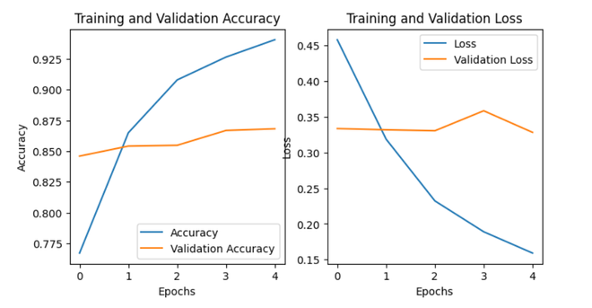
Plot of training and validation accuracy and loss

The code visualizes the training and validation accuracy as well as the training and validation loss over epochs. It extracts accuracy and loss values from the training history (history_dict). The matplotlib library is then used to create a side-by-side subplot, where the left subplot displays accuracy trends, and the right subplot shows loss trends over epochs.

5. Testing the trained model

Now, we will test the trained model with a random review and check its output.

Python3

# Making predictions
sample_text = (
    '''The movie by GeeksforGeeks was so good and the animation are so dope.
    I would recommend my friends to watch it.'''
)
predictions = model.predict(np.array([sample_text]))
print(*predictions[0])

# Print the label based on the prediction
if predictions[0] > 0:
    print('The review is positive')
else:
    print('The review is negative')

Output:

1/1 [==============================] - 0s 33ms/step
5.414222
The review is positive

The code makes predictions on a sample text using the trained model (model.predict(np.array([sample_text]))). The result (predictions[0]) represents the model’s confidence in the sentiment, where positive values indicate a positive sentiment and negative values indicate a negative sentiment. The subsequent conditional statement interprets the prediction, printing either ‘The review is positive’ or ‘The review is negative’ based on the model’s classification.

Advantages and Disadvantages of RNN for Text Classifications in NLP

Advantages

When it comes to natural language processing (NLP) text categorization tasks, recurrent neural networks (RNNs) provide the following benefits:

• Sequential Information Processing: Because they are built to handle sequences, RNNs work well in jobs where the order in which the input data is entered is important. RNNs are very good at capturing the contextual links between words in a sentence, which is important in text categorization when word order affects meaning.
• Variable-length Input: Sequences of different lengths can be processed by RNNs. Since text documents in NLP might vary in length, this flexibility is especially helpful. RNNs analyze a variety of textual data types efficiently because they dynamically adjust to the size of the input.
• Feature Learning: From the input data, RNNs automatically extract pertinent features and representations. This helps the model recognize significant patterns and relationships in the text for text classification, which lessens the requirement for human feature engineering.

Disadvantages

For text categorization tasks in Natural Language Processing (NLP), Recurrent Neural Networks (RNNs) have certain drawbacks despite their benefits:

• Vanishing Gradient Problem: RNNs are prone to the vanishing gradient problem, where gradients diminish exponentially as they are propagated back through time. This can result in difficulties in learning long-term dependencies in sequences, limiting the model’s ability to capture context over extended distances.
• Limited Parallelization: RNNs process sequences sequentially, making it challenging to parallelize computations. This lack of parallelization can lead to slower training times compared to other architectures, such as convolutional neural networks (CNNs), especially for long sequences.
• Sensitivity to Input Order: RNNs are sensitive to the order of inputs, and slight variations in input order can result in different model outputs. This sensitivity might make the model less robust, particularly in situations where slight variations in word order do not significantly alter the intended meaning.

Frequently Asked Questions (FAQs)

1. What is an RNN, and how does it differ from other neural network architectures?

RNNs are a type of neural network designed for sequence data. Unlike traditional feedforward networks, RNNs have connections that form a directed cycle, allowing them to maintain a memory of previous inputs. This makes them suitable for tasks involving sequences, such as text data.

2. How does an RNN handle sequential information in text classification?

RNNs process text sequentially, considering the order of words. Each word’s representation depends not only on the current word but also on the context of preceding words, enabling the model to capture sequential dependencies crucial for understanding text.

3. What are the common challenges faced by RNNs in text classification?

RNNs face challenges such as the vanishing gradient problem, difficulty in capturing long-term dependencies, and sensitivity to input order. These challenges can impact the model’s ability to effectively learn from and classify text data.

4. How can the vanishing gradient problem be mitigated in RNNs?

The vanishing gradient problem in RNNs can be addressed using advanced architectures like Long Short-Term Memory (LSTM) networks and Gated Recurrent Unit (GRU) networks. These architectures incorporate mechanisms to selectively retain and update information over longer sequences.

5. How to use an RNN for text classification in NLP?

To use an RNN for text classification in NLP, preprocess text data by tokenizing and converting it to numerical format. Build an RNN model with layers like embedding, recurrent, and dense layers, then compile it with a suitable loss function and optimizer. Train the model on labeled data, evaluate its performance, and make predictions on new text for classification tasks.