ML | Rainfall prediction using Linear regression
Last Updated :
03 Mar, 2023
Rainfall prediction is a common application of machine learning, and linear regression is a simple and effective technique that can be used for this purpose. In this task, the goal is to predict the amount of rainfall based on historical data.
Linear regression is a supervised learning algorithm that is used to model the relationship between a dependent variable and one or more independent variables. In this case, the dependent variable is the amount of rainfall, and the independent variables are the features that are used to predict it, such as temperature, humidity, wind speed, etc.
The first step is to collect the historical data, which includes the amount of rainfall and the corresponding values of the independent variables. Once the data has been collected, it needs to be cleaned and preprocessed to remove any outliers or missing values.
Next, the data is split into two sets: the training set and the testing set. The training set is used to train the model, while the testing set is used to evaluate its performance.
To perform linear regression, we need to first define a hypothesis function that maps the input variables to the output variable. In this case, the hypothesis function is a linear equation of the form:
y = b0 + b1x1 + b2x2 + … + bnxn
where y is the predicted amount of rainfall, x1, x2, …, xn are the input variables, and b0, b1, b2, …, bn are the coefficients that are learned during training.
To train the model, we need to find the values of the coefficients that minimize the difference between the predicted values and the actual values in the training set. This is done by minimizing the mean squared error (MSE) using gradient descent or some other optimization algorithm.
Once the model has been trained, it can be used to predict the amount of rainfall for new input values. The performance of the model can be evaluated using various metrics such as the coefficient of determination (R^2), mean squared error (MSE), and root mean squared error (RMSE).
In summary, linear regression is a simple and effective technique that can be used to predict the amount of rainfall based on historical data. The process involves collecting and preprocessing the data, defining a hypothesis function, training the model, and evaluating its performance.
Prerequisites: Linear regression
Rainfall Prediction is the application of science and technology to predict the amount of rainfall over a region. It is important to exactly determine the rainfall for the effective use of water resources, crop productivity and pre-planning of water structures. In this article, we will use Linear Regression to predict the amount of rainfall. Linear Regression tells us how many inches of rainfall we can expect. The dataset is a public weather dataset from Austin, Texas available on Kaggle. The dataset can be found here.
Data Cleaning: Data comes in all forms, most of it is very messy and unstructured. They rarely come ready to use. Datasets, large and small, come with a variety of issues- invalid fields, missing and additional values, and values that are in forms different from the ones we require. In order to bring it to a workable or structured form, we need to “clean” our data, and make it ready to use. Some common cleaning includes parsing, converting to one-hot, removing unnecessary data, etc. In our case, our data has some days where some factors weren’t recorded. And the rainfall in cm was marked as T if there was trace precipitation. Our algorithm requires numbers, so we can’t work with alphabets popping up in our data. so we need to clean the data before applying it to our model Cleaning the data in Python:
Python3
import pandas as pd
import numpy as np
data = pd.read_csv(& quot
austin_weather.csv & quot
)
data = data.drop(['Events', 'Date', 'SeaLevelPressureHighInches',
'SeaLevelPressureLowInches'], axis=1)
data = data.replace('T', 0.0)
data = data.replace('-', 0.0)
data.to_csv('austin_final.csv')
|
Once the data is cleaned, it can be used as input to our Linear regression model. Linear regression is a linear approach to forming a relationship between a dependent variable and many independent explanatory variables. This is done by plotting a line that fits our scatter plot the best, ie, with the least errors. This gives value predictions, ie, how much, by substituting the independent values in the line equation. We will use Scikit-learn’s linear regression model to train our dataset. Once the model is trained, we can give our own inputs for the various columns such as temperature, dew point, pressure, etc. to predict the weather based on these attributes.
python3
import pandas as pd
import numpy as np
import sklearn as sk
from sklearn.linear_model import LinearRegression
import matplotlib.pyplot as plt
data = pd.read_csv("austin_final.csv")
X = data.drop(['PrecipitationSumInches'], axis=1)
Y = data['PrecipitationSumInches']
Y = Y.values.reshape(-1, 1)
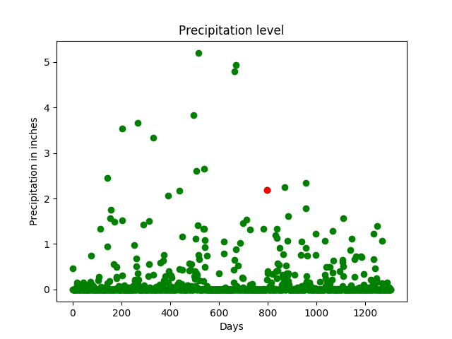
day_index = 798
days = [i for i in range(Y.size)]
clf = LinearRegression()
clf.fit(X, Y)
inp = np.array([[74], [60], [45], [67], [49], [43], [33], [45],
[57], [29.68], [10], [7], [2], [0], [20], [4], [31]])
inp = inp.reshape(1, -1)
print('The precipitation in inches for the input is:', clf.predict(inp))
print("the precipitation trend graph: ")
plt.scatter(days, Y, color='g')
plt.scatter(days[day_index], Y[day_index], color='r')
plt.title("Precipitation level")
plt.xlabel("Days")
plt.ylabel("Precipitation in inches")
plt.show()
x_vis = X.filter(['TempAvgF', 'DewPointAvgF', 'HumidityAvgPercent',
'SeaLevelPressureAvgInches', 'VisibilityAvgMiles',
'WindAvgMPH'], axis=1)
print("Precipitation vs selected attributes graph: ")
for i in range(x_vis.columns.size):
plt.subplot(3, 2, i + 1)
plt.scatter(days, x_vis[x_vis.columns.values[i][:100]],
color='g')
plt.scatter(days[day_index],
x_vis[x_vis.columns.values[i]][day_index],
color='r')
plt.title(x_vis.columns.values[i])
plt.show()
|
Output :
The precipitation in inches for the input is: [[1.33868402]]

The precipitation trend graph:
Precipitation vs selected attributes graph:
A day (in red) having precipitation of about 2 inches is tracked across multiple parameters (the same day is tracker across multiple features such as temperature, pressure, etc). The x-axis denotes the days and the y-axis denotes the magnitude of the feature such as temperature, pressure, etc. From the graph, it can be observed that rainfall can be expected to be high when the temperature is high and humidity is high.
Share your thoughts in the comments
Please Login to comment...