Knowing the complexity in competitive programming
Last Updated :
06 Dec, 2023
Prerequisite: Time Complexity Analysis
Generally, while doing competitive programming problems on various sites, the most difficult task faced is writing the code under desired complexity otherwise the program will get a TLE (Time Limit Exceeded).
A naive solution is almost never accepted. So how to know, what complexity is acceptable?
The answer to this question is directly related to the number of operations that are allowed to perform within a second. Most of the sites these days allow 108 operations per second, only a few sites still allow 107 operations. After figuring out the number of operations that can be performed, search for the right complexity by looking at the constraints given in the problem.
Example: Given an array A[] and a number x, check for a pair in A[] with the sum as x, where N is:
1) 1 <= N <= 103
2) 1 <= N <= 105
3) 1 <= N <= 108
- For Case 1: A naive solution that is using two for-loops works as it gives us a complexity of O(N2), which even in the worst case will perform 106 operations which are well under 108. Of course, O(N) and O(NlogN) is also acceptable in this case.
- For Case 2: We have to think of a better solution than O(N2), as in worst case, it will perform 1010 operations as N is 105. So complexity acceptable for this case is either O(NlogN) which is approximately 106 (105 * ~10) operations well under 108 or O(N).
- For Case 3: Even O(NlogN) gives us TLE as it performs ~109 operations which are over 108. So, the only solution which is acceptable is O(N) which in worst case will perform 10^8 operations. The code for the given problem can be found on : https://www.geeksforgeeks.org/write-a-c-program-that-given-a-set-a-of-n-numbers-and-another-number-x-determines-whether-or-not-there-exist-two-elements-in-s-whose-sum-is-exactly-x/
Estimating efficiency:
Given: The time limit for a problem is 1 second.
The input size for the problem is 105.
And, if the Time complexity is O(n2)
So, the Algorithm will perform about (105)2 = 1010 number of operation
This should take at least 10 seconds, The algorithm seems to be too slow for solving the problem.
How to Determine the solution of a problem by looking at its constraints?
So, in our previous example given input size n=105, it is probably expected that the time complexity of the algorithm is O(n) or O(n logn).
That is how this can help us to design the algorithm easier because it rules out approaches that would yield an algorithm with a worse time complexity.
It is important to remember that time complexity is only an estimate of efficiency because it hides the constant factors. For example, an algorithm that runs in O(n) time may perform n/2 or 2n operations.
Let’s discuss the classic problem for a better understanding of time complexity Estimating efficiency,
Given an array of n numbers, our task is to calculate the maximum subarray sum. The largest possible sum of a sequence of consecutive values in the array.
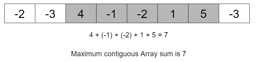
The largest possible sum of a sequence of consecutive values in the array.
This problem has a straightforward O(n3) solution however, by designing a better algorithm, it is possible to solve the problem in O(n2) time and even in O(n) time.
Method number 1:-
In this method, we go through all possible subarrays, calculate the sum of values in each subarray and maintain the maximum sum.
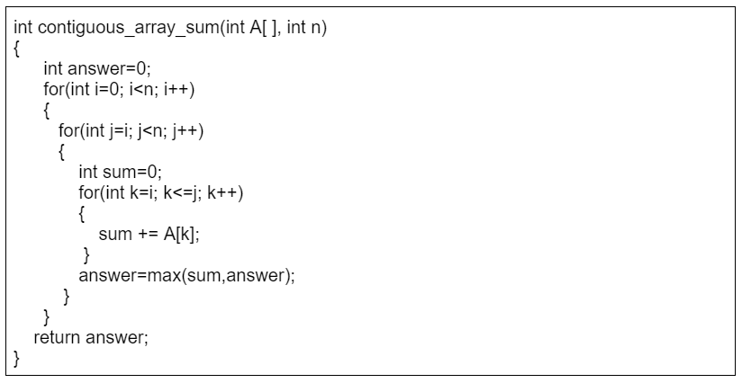
Algorithm 1 with time complexity O(n3)
The variables i and j fix the first and last index of the subarray, and the sum of values is calculated to the variable sum. The variable answer contains the maximum sum found during the search.
Time complexity – O(n3), because it consists of three nested loops.
Method number 2:-
It is really easy to make method number 1 more efficient by removing one loop from it. This is possible by calculating the sum at the same time when the right end of the subarray moves.
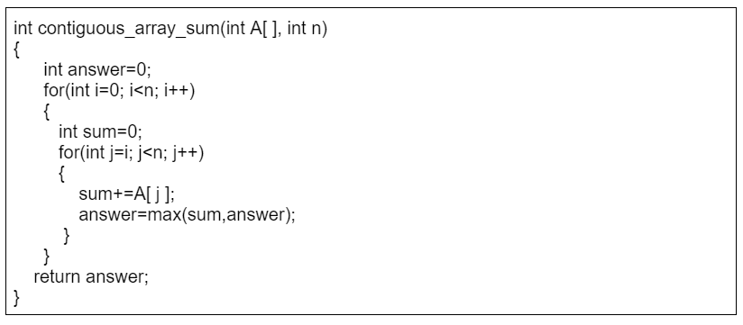
Algorithm 2 with time complexity O(n2)
Time complexity – O(n2), because it consists of two nested loops.
Method number 3:-
Surprisingly, it is possible to solve the problem in O(n) time, which means that just one loop is enough. The idea is to calculate, for each array position, the maximum sum of a subarray that ends at that position. After this, the answer to the problem is the maximum of those sums.
The subproblem of finding the maximum-sum subarray that ends at position ith. There are two possibilities:
1. The subarray only contains the element at position ith.
2. The subarray consists of a subarray that ends at position i −1, followed by the element at position i.
As we want to find a subarray with the maximum sum, the subarray that ends at position i −1 should also have the maximum sum. Thus, we can solve the problem efficiently by calculating the maximum subarray sum for each ending position from left to right.
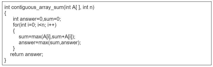
Algorithm 3 with time complexity O(n)
Time complexity – O(n), because it consists of one loop, This is also the best possible time complexity, because any algorithm for the problem has to examine all array elements at least once.
Let’s compare all these three methods against all possible given input sizes and see their execution time:
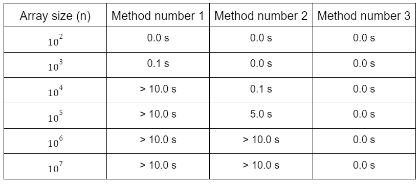
compare different methods/Algorithm with different Array sizes
It is interesting to see how efficient algorithms are in practice. The above table shows the running times of the above algorithms/methods for different values of n.
The comparison shows that all algorithms are efficient when the input size is small, but larger inputs bring out remarkable differences in the running times of the algorithms.
Method 1 becomes slow when n = 104, and method 2 starts to become slow when n = 105. Only method 3 is able to process even the largest inputs instantly.
Share your thoughts in the comments
Please Login to comment...