Introduction to Residual Networks

Recent years have seen tremendous progress in the field of Image Processing and Recognition. Deep Neural Networks are becoming deeper and more complex. It has been proved that adding more layers to a Neural Network can make it more robust for image-related tasks. But it can also cause them to lose accuracy. That’s where Residual Networks come into place.

The tendency to add so many layers by deep learning practitioners is to extract important features from complex images. So, the first layers may detect edges, and the subsequent layers at the end may detect recognizable shapes, like tires of a car. But if we add more than 30 layers to the network, then its performance suffers and it attains a low accuracy. This is contrary to the thinking that the addition of layers will make a neural network better. This is not due to overfitting, because in that case, one may use dropout and regularization techniques to solve the issue altogether. It’s mainly present because of the popular vanishing gradient problem.

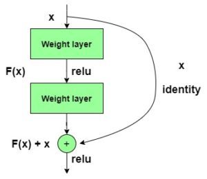
y = F(x) + x

The ResNet152 model with 152 layers won the ILSVRC Imagenet 2015 test while having lesser parameters than the VGG19 network, which was very popular at that time. A residual network consists of residual units or blocks which have skip connections, also called identity connections.

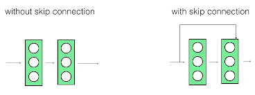
The skip connections are shown below:

The output of the previous layer is added to the output of the layer after it in the residual block. The hop or skip could be 1, 2 or even 3. When adding, the dimensions of x may be different than F(x) due to the convolution process, resulting in a reduction of its dimensions. Thus, we add an additional 1 x 1 convolution layer to change the dimensions of x.

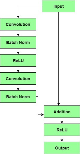
A residual block has a 3 x 3 convolution layer followed by a batch normalization layer and a ReLU activation function. This is again continued by a 3 x 3 convolution layer and a batch normalization layer. The skip connection basically skips both these layers and adds directly before the ReLU activation function. Such residual blocks are repeated to form a residual network.

After an in-depth comparison of all the present CNN architectures was done, the ResNet stood out by holding the lowest top 5% error rate at 3.57% for classification tasks, overtaking all the other architectures. Even humans do not have much lower error rates.

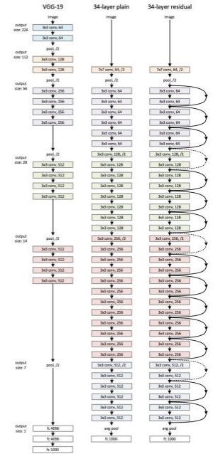
Comparison of 34 layer ResNet with VGG19 and a 34 layer plain network:

To conclude, it can be said that residual networks have become quite popular for image recognition and classification tasks because of their ability to solve vanishing and exploding gradients when adding more layers to an already deep neural network. A ResNet with thousand layers has not much practical use as of now.

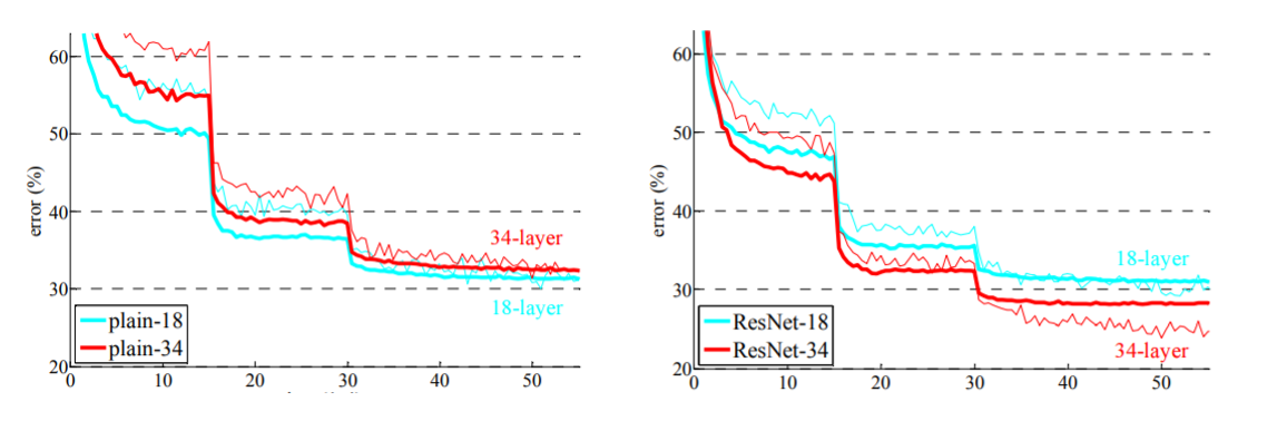
The below graphs compare the accuracies of a plain network with that of a residual network. Note that with increasing layers a 34-layer plain network’s accuracy starts to saturate earlier than ResNet’s accuracy.