Deep Convolutional GAN with Keras

Deep Convolutional GAN (DCGAN) was proposed by a researcher from MIT and Facebook AI research. It is widely used in many convolution-based generation-based techniques. The focus of this paper was to make training GANs stable. Hence, they proposed some architectural changes in the computer vision problems. In this article, we will be using DCGAN on the fashion MNIST dataset to generate images related to clothes.

Need for DCGANs:

DCGANs are introduced to reduce the problem of mode collapse. Mode collapse occurs when the generator got biased towards a few outputs and can’t able to produce outputs of every variation from the dataset. For example- take the case of mnist digits dataset (digits from 0 to 9) , we want the generator should generate all type of digits but sometimes our generator got biased towards two to three digits and produce them only. Because of that the discriminator also got optimized towards that particular digits only, and this state is known as mode collapse. But this problem can be overcome by using DCGANs.

Architecture:

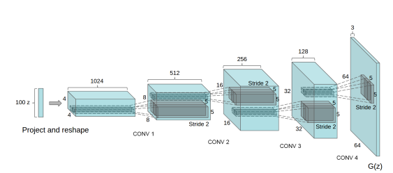
The generator of the DCGAN architecture takes 100 uniform generated values using normal distribution as an input. First, it changes the dimension to 4x4x1024 and performed a fractionally stridden convolution 4 times with a stride of 1/2 (this means every time when applied, it doubles the image dimension while reducing the number of output channels). The generated output has dimensions of (64, 64, 3). There are some architectural changes proposed in the generator such as the removal of all fully connected layers, and the use of Batch Normalization which helps in stabilizing training.  In this paper, the authors use ReLU activation function in all layers of the generator, except for the output layers. We will be implementing generator with similar guidelines but not completely the same architecture.

The role of the discriminator here is to determine that the image comes from either a real dataset or a generator. The discriminator can be simply designed similar to a convolution neural network that performs an image classification task. However, the authors of this paper suggested some changes in the discriminator architecture. Instead of fully connected layers, they used only strided-convolutions with LeakyReLU as an activation function, the input of the generator is a single image from the dataset or generated image and the output is a score that determines whether the image is real or generated.

Implementation:

In this section we will be discussing the implementation of DCGAN in Keras, since our dataset in the Fashion MNIST dataset, this dataset contains images of size (28, 28) of 1 color channel instead of (64, 64) of 3 color channels. So, we need to make some changes in the architecture, we will be discussing these changes as we go along.

In the first step, we need to import the necessary classes such as TensorFlow, Keras, matplotlib, etc. We will be using TensorFlow version 2.  This version of TensorFlow provides inbuilt support for the Keras library as its default High-level API.

python3

# code % matplotlib inline
import tensorflow as tf
from tensorflow import keras
import numpy as np
import matplotlib.pyplot as plt
from tqdm import tqdm
from IPython import display

# Check tensorflow version
print('Tensorflow version:', tf.__version__)

Now we load the fashion-MNIST dataset, the good thing is that the dataset can be imported from tf.keras.datasets API. So, we don’t need to load datasets manually by copying files. This dataset contains 60k training images and 10k test images for each dimension (28, 28, 1). Since the value of each pixel is in the range (0, 255), we divide these values by 255 to normalize it.

python3

(x_train, y_train), (x_test, y_test) = tf.keras.datasets.fashion_mnist.load_data()
x_train = x_train.astype(np.float32) / 255.0
x_test = x_test.astype(np.float32) / 255.0
x_train.shape, x_test.shape

((60000, 28, 28), (10000, 28, 28))

Now in the next step, we will be visualizing some of the images from the Fashion-MNIST dataset, we use matplotlib library for that.

python3

# We plot first 25 images of training dataset
plt.figure(figsize =(10, 10))
for i in range(25):
    plt.subplot(5, 5, i + 1)
    plt.xticks([])
    plt.yticks([])
    plt.grid(False)
    plt.imshow(x_train[i], cmap = plt.cm.binary)
plt.show()

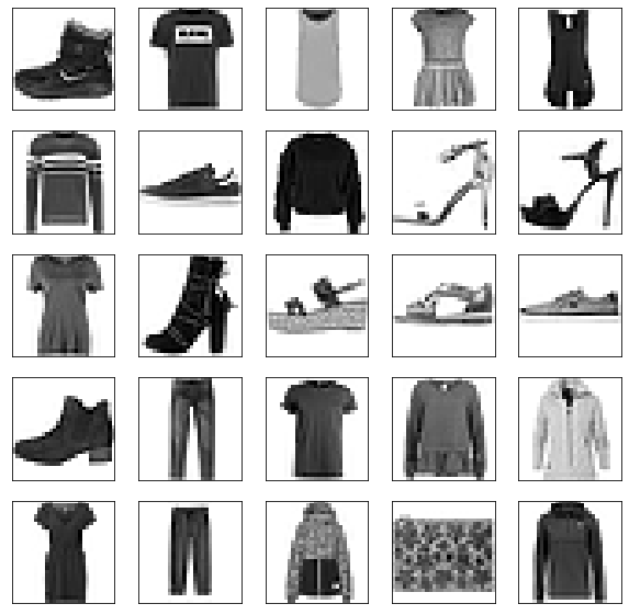
Original Fashion MNIST images

Now, we define training parameters such as batch size and divide the dataset into batches, and fill those batches by randomly sampling the training data.

python3

# code
batch_size = 32
# This dataset fills a buffer with buffer_size elements,
# then randomly samples elements from this buffer,
# replacing the selected elements with new elements.
def create_batch(x_train):
  dataset = tf.data.Dataset.from_tensor_slices(x_train).shuffle(1000)
  # Combines consecutive elements of this dataset into batches.

  dataset = dataset.batch(batch_size, drop_remainder = True).prefetch(1)
  # Creates a Dataset that prefetches elements from this dataset
  return dataset

Now, we define the generator architecture, this generator architecture takes a vector of size 100 and first reshape that into (7, 7, 128) vector and then, it applies transpose convolution on that reshaped image in combination with batch normalization. The output of this generator is a trained image of dimension (28, 28, 1).

python3

# code
num_features = 100

generator = keras.models.Sequential([
    keras.layers.Dense(7 * 7 * 128, input_shape =[num_features]),
    keras.layers.Reshape([7, 7, 128]),
    keras.layers.BatchNormalization(),
    keras.layers.Conv2DTranspose(
        64, (5, 5), (2, 2), padding ="same", activation ="selu"),
    keras.layers.BatchNormalization(),
    keras.layers.Conv2DTranspose(
        1, (5, 5), (2, 2), padding ="same", activation ="tanh"),
])
generator.summary()

Model: "sequential"
_________________________________________________________________
Layer (type)                 Output Shape              Param #   
=================================================================
dense (Dense)                (None, 6272)              633472    
_________________________________________________________________
reshape (Reshape)            (None, 7, 7, 128)         0         
_________________________________________________________________
batch_normalization (BatchNo (None, 7, 7, 128)         512       
_________________________________________________________________
conv2d_transpose (Conv2DTran (None, 14, 14, 64)        204864    
_________________________________________________________________
batch_normalization_1 (Batch (None, 14, 14, 64)        256       
_________________________________________________________________
conv2d_transpose_1 (Conv2DTr (None, 28, 28, 1)         1601      
=================================================================
Total params: 840, 705
Trainable params: 840, 321
Non-trainable params: 384
_________________________________________________________________

Now, we define discriminator architecture, the discriminator takes an image of size  28*28 with 1 color channel and outputs a scalar value representing an image from either dataset or generated image.

python3

discriminator = keras.models.Sequential([
    keras.layers.Conv2D(64, (5, 5), (2, 2), padding ="same", input_shape =[28, 28, 1]),
    keras.layers.LeakyReLU(0.2),
    keras.layers.Dropout(0.3),
    keras.layers.Conv2D(128, (5, 5), (2, 2), padding ="same"),
    keras.layers.LeakyReLU(0.2),
    keras.layers.Dropout(0.3),
    keras.layers.Flatten(),
    keras.layers.Dense(1, activation ='sigmoid')
])
discriminator.summary()

Model: "sequential_1"
_________________________________________________________________
Layer (type)                 Output Shape              Param #   
=================================================================
conv2d (Conv2D)              (None, 14, 14, 64)        1664      
_________________________________________________________________
leaky_re_lu (LeakyReLU)      (None, 14, 14, 64)        0         
_________________________________________________________________
dropout (Dropout)            (None, 14, 14, 64)        0         
_________________________________________________________________
conv2d_1 (Conv2D)            (None, 7, 7, 128)         204928    
_________________________________________________________________
leaky_re_lu_1 (LeakyReLU)    (None, 7, 7, 128)         0         
_________________________________________________________________
dropout_1 (Dropout)          (None, 7, 7, 128)         0         
_________________________________________________________________
flatten (Flatten)            (None, 6272)              0         
_________________________________________________________________
dense_1 (Dense)              (None, 1)                 6273      
=================================================================
Total params: 212, 865
Trainable params: 212, 865
Non-trainable params: 0
_________________________________________________________________

Now we need to compile our DCGAN model (combination of generator and discriminator), we will first compile the discriminator and set its training to False, because we first want to train the generator.

python3

# compile discriminator using binary cross entropy loss and adam optimizer
discriminator.compile(loss ="binary_crossentropy", optimizer ="adam")
# make  discriminator no-trainable as of  now
discriminator.trainable = False
# Combine both generator and discriminator
gan = keras.models.Sequential([generator, discriminator])
# compile generator using binary cross entropy loss and adam optimizer

gan.compile(loss ="binary_crossentropy", optimizer ="adam")

Now, we define the training procedure for this GAN model, we will be using tqdm package which we have imported earlier., this package helps in visualizing training.

python3

seed = tf.random.normal(shape =[batch_size, 100])

def train_dcgan(gan, dataset, batch_size, num_features, epochs = 5):
    generator, discriminator = gan.layers
    for epoch in tqdm(range(epochs)):
        print()
        print("Epoch {}/{}".format(epoch + 1, epochs))

        for X_batch in dataset:
            # create a random noise of sizebatch_size * 100
            # to passit into the generator
            noise = tf.random.normal(shape =[batch_size, num_features])
            generated_images = generator(noise)

            # take batch of generated image and real image and
            #  use them to train  the discriminator
            X_fake_and_real = tf.concat([generated_images, X_batch], axis = 0)
            y1 = tf.constant([[0.]] * batch_size + [[1.]] * batch_size)
            discriminator.trainable = True
            discriminator.train_on_batch(X_fake_and_real, y1)

            # Here we will be training our GAN model, in this step
            #  we pass noise that uses generatortogenerate the image
            #  and pass it with labels as [1] So, it can fool the discriminator
            noise = tf.random.normal(shape =[batch_size, num_features])
            y2 = tf.constant([[1.]] * batch_size)
            discriminator.trainable = False
            gan.train_on_batch(noise, y2)

            # generate images for the GIF as we go
            generate_and_save_images(generator, epoch + 1, seed)

    generate_and_save_images(generator, epochs, seed)

Now we define a function that generates and save images from generator (during training). We will use these generated images to plot the GIF later.

python3

# code
def generate_and_save_images(model, epoch, test_input):
  predictions = model(test_input, training = False)

  fig = plt.figure(figsize =(10, 10))

  for i in range(25):
      plt.subplot(5, 5, i + 1)
      plt.imshow(predictions[i, :, :, 0] * 127.5 + 127.5, cmap ='binary')
      plt.axis('off')

  plt.savefig('image_epoch_{:04d}.png'.format(epoch))

Now, we need to train the model but before that, we also need to create batches of training data and add a dimension that represents number of color maps.

python3

# reshape to add a color map
x_train_dcgan = x_train.reshape(-1, 28, 28, 1) * 2. - 1.
# create batches
dataset = create_batch(x_train_dcgan)
# callthe training function with 10 epochs and record time %% time
train_dcgan(gan, dataset, batch_size, num_features, epochs = 10)

0%|          | 0/10 [00:00<?, ?it/s]
Epoch 1/10

 10%|?         | 1/10 [01:04<09:39, 64.37s/it]
Epoch 2/10

 20%|??        | 2/10 [02:10<08:39, 64.99s/it]
Epoch 3/10

 30%|???       | 3/10 [03:14<07:33, 64.74s/it]
Epoch 4/10

 40%|????      | 4/10 [04:19<06:27, 64.62s/it]
Epoch 5/10

 50%|?????     | 5/10 [05:23<05:22, 64.58s/it]
Epoch 6/10

 60%|??????    | 6/10 [06:27<04:17, 64.47s/it]
Epoch 7/10

 70%|???????   | 7/10 [07:32<03:13, 64.55s/it]
Epoch 8/10

 80%|????????  | 8/10 [08:37<02:08, 64.48s/it]
Epoch 9/10

 90%|????????? | 9/10 [09:41<01:04, 64.54s/it]
Epoch 10/10

100%|??????????| 10/10 [10:46<00:00, 64.61s/it]
CPU times: user 7min 4s, sys: 33.3 s, total: 7min 37s
Wall time: 10min 46s

Now we will define a function that takes the saved images and convert them into GIF. We use this function from here

python3

import imageio
import glob

anim_file = 'dcgan_results.gif'

with imageio.get_writer(anim_file, mode ='I') as writer:
  filenames = glob.glob('image*.png')
  filenames = sorted(filenames)
  last = -1
  for i, filename in enumerate(filenames):
    frame = 2*(i)
    if round(frame) > round(last):
      last = frame
    else:
      continue
    image = imageio.imread(filename)
    writer.append_data(image)
  image = imageio.imread(filename)
  writer.append_data(image)
display.Image(filename = anim_file)

Generated Images results

Results and Conclusion:

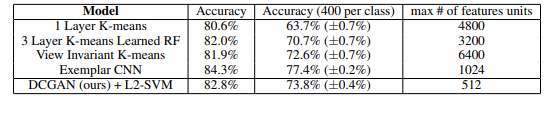
To evaluate the quality of the representations learned by DCGANs for supervised tasks, the authors train the model on ImageNet-1k and then use the discriminator’s convolution features from all layers, max-pooling each layer’s representation to produce a 4 × 4 spatial grid. These features are then flattened and concatenated to form a 28672-dimensional vector and a regularized linear L2-SVM classifier is trained on top of them.  This model is then evaluated on CIFAR-10 dataset but not trained on it. The model reported an accuracy of 82 % which also displays the robustness of the model.

On Street View Housing Number dataset, it achieved a validation loss of 22% which is the new state-of-the-art, even discriminator architecture when supervise and trained as a CNN model has more validation loss than it.