A Naive Bayes classifiers, a family of algorithms based on Bayes’ Theorem. Despite the “naive” assumption of feature independence, these classifiers are widely utilized for their simplicity and efficiency in machine learning. The article delves into theory, implementation, and applications, shedding light on their practical utility despite oversimplified assumptions.
What is Naive Bayes Classifiers?
Naive Bayes classifiers are a collection of classification algorithms based on Bayes’ Theorem. It is not a single algorithm but a family of algorithms where all of them share a common principle, i.e. every pair of features being classified is independent of each other. To start with, let us consider a dataset.
One of the most simple and effective classification algorithms, the Naïve Bayes classifier aids in the rapid development of machine learning models with rapid prediction capabilities.
Naïve Bayes algorithm is used for classification problems. It is highly used in text classification. In text classification tasks, data contains high dimension (as each word represent one feature in the data). It is used in spam filtering, sentiment detection, rating classification etc. The advantage of using naïve Bayes is its speed. It is fast and making prediction is easy with high dimension of data.
This model predicts the probability of an instance belongs to a class with a given set of feature value. It is a probabilistic classifier. It is because it assumes that one feature in the model is independent of existence of another feature. In other words, each feature contributes to the predictions with no relation between each other. In real world, this condition satisfies rarely. It uses Bayes theorem in the algorithm for training and prediction
Why it is Called Naive Bayes?
The “Naive” part of the name indicates the simplifying assumption made by the Naïve Bayes classifier. The classifier assumes that the features used to describe an observation are conditionally independent, given the class label. The “Bayes” part of the name refers to Reverend Thomas Bayes, an 18th-century statistician and theologian who formulated Bayes’ theorem.
Consider a fictional dataset that describes the weather conditions for playing a game of golf. Given the weather conditions, each tuple classifies the conditions as fit(“Yes”) or unfit(“No”) for playing golf.Here is a tabular representation of our dataset.
| | Outlook | Temperature | Humidity | Windy | Play Golf |
|---|
| 0 | Rainy | Hot | High | False | No |
| 1 | Rainy | Hot | High | True | No |
| 2 | Overcast | Hot | High | False | Yes |
| 3 | Sunny | Mild | High | False | Yes |
| 4 | Sunny | Cool | Normal | False | Yes |
| 5 | Sunny | Cool | Normal | True | No |
| 6 | Overcast | Cool | Normal | True | Yes |
| 7 | Rainy | Mild | High | False | No |
| 8 | Rainy | Cool | Normal | False | Yes |
| 9 | Sunny | Mild | Normal | False | Yes |
| 10 | Rainy | Mild | Normal | True | Yes |
| 11 | Overcast | Mild | High | True | Yes |
| 12 | Overcast | Hot | Normal | False | Yes |
| 13 | Sunny | Mild | High | True | No |
The dataset is divided into two parts, namely, feature matrix and the response vector.
- Feature matrix contains all the vectors(rows) of dataset in which each vector consists of the value of dependent features. In above dataset, features are ‘Outlook’, ‘Temperature’, ‘Humidity’ and ‘Windy’.
- Response vector contains the value of class variable(prediction or output) for each row of feature matrix. In above dataset, the class variable name is ‘Play golf’.
Assumption of Naive Bayes
The fundamental Naive Bayes assumption is that each feature makes an:
- Feature independence: The features of the data are conditionally independent of each other, given the class label.
- Continuous features are normally distributed: If a feature is continuous, then it is assumed to be normally distributed within each class.
- Discrete features have multinomial distributions: If a feature is discrete, then it is assumed to have a multinomial distribution within each class.
- Features are equally important: All features are assumed to contribute equally to the prediction of the class label.
- No missing data: The data should not contain any missing values.
With relation to our dataset, this concept can be understood as:
- We assume that no pair of features are dependent. For example, the temperature being ‘Hot’ has nothing to do with the humidity or the outlook being ‘Rainy’ has no effect on the winds. Hence, the features are assumed to be independent.
- Secondly, each feature is given the same weight(or importance). For example, knowing only temperature and humidity alone can’t predict the outcome accurately. None of the attributes is irrelevant and assumed to be contributing equally to the outcome.
The assumptions made by Naive Bayes are not generally correct in real-world situations. In-fact, the independence assumption is never correct but often works well in practice.Now, before moving to the formula for Naive Bayes, it is important to know about Bayes’ theorem.
Bayes’ Theorem
Bayes’ Theorem finds the probability of an event occurring given the probability of another event that has already occurred. Bayes’ theorem is stated mathematically as the following equation:
[Tex] P(A|B) = \frac{P(B|A) P(A)}{P(B)}
[/Tex]
where A and B are events and P(B) ≠ 0
- Basically, we are trying to find probability of event A, given the event B is true. Event B is also termed as evidence.
- P(A) is the priori of A (the prior probability, i.e. Probability of event before evidence is seen). The evidence is an attribute value of an unknown instance(here, it is event B).
- P(B) is Marginal Probability: Probability of Evidence.
- P(A|B) is a posteriori probability of B, i.e. probability of event after evidence is seen.
- P(B|A) is Likelihood probability i.e the likelihood that a hypothesis will come true based on the evidence.
Now, with regards to our dataset, we can apply Bayes’ theorem in following way:
[Tex] P(y|X) = \frac{P(X|y) P(y)}{P(X)}
[/Tex]
where, y is class variable and X is a dependent feature vector (of size n) where:
[Tex] X = (x_1,x_2,x_3,…..,x_n)
[/Tex]
Just to clear, an example of a feature vector and corresponding class variable can be: (refer 1st row of dataset)
X = (Rainy, Hot, High, False)
y = No
So basically, [Tex]P(y|X)
[/Tex]here means, the probability of “Not playing golf” given that the weather conditions are “Rainy outlook”, “Temperature is hot”, “high humidity” and “no wind”.
With relation to our dataset, this concept can be understood as:
- We assume that no pair of features are dependent. For example, the temperature being ‘Hot’ has nothing to do with the humidity or the outlook being ‘Rainy’ has no effect on the winds. Hence, the features are assumed to be independent.
- Secondly, each feature is given the same weight(or importance). For example, knowing only temperature and humidity alone can’t predict the outcome accurately. None of the attributes is irrelevant and assumed to be contributing equally to the outcome.
Now, its time to put a naive assumption to the Bayes’ theorem, which is, independence among the features. So now, we split evidence into the independent parts.
Now, if any two events A and B are independent, then,
P(A,B) = P(A)P(B)
Hence, we reach to the result:
[Tex] P(y|x_1,…,x_n) = \frac{ P(x_1|y)P(x_2|y)…P(x_n|y)P(y)}{P(x_1)P(x_2)…P(x_n)}
[/Tex]
which can be expressed as:
[Tex] P(y|x_1,…,x_n) = \frac{P(y)\prod_{i=1}^{n}P(x_i|y)}{P(x_1)P(x_2)…P(x_n)}
[/Tex]
Now, as the denominator remains constant for a given input, we can remove that term:
[Tex] P(y|x_1,…,x_n)\propto P(y)\prod_{i=1}^{n}P(x_i|y)
[/Tex]
Now, we need to create a classifier model. For this, we find the probability of given set of inputs for all possible values of the class variable y and pick up the output with maximum probability. This can be expressed mathematically as:
[Tex]y = argmax_{y} P(y)\prod_{i=1}^{n}P(x_i|y)
[/Tex]
So, finally, we are left with the task of calculating [Tex] P(y)
[/Tex]and [Tex]P(x_i | y)
[/Tex].
Please note that [Tex]P(y)
[/Tex] is also called class probability and [Tex]P(x_i | y)
[/Tex] is called conditional probability.
The different naive Bayes classifiers differ mainly by the assumptions they make regarding the distribution of [Tex]P(x_i | y).
[/Tex]
Let us try to apply the above formula manually on our weather dataset. For this, we need to do some precomputations on our dataset.
We need to find[Tex] P(x_i | y_j)
[/Tex]for each [Tex]x_i
[/Tex] in X and[Tex]y_j
[/Tex] in y. All these calculations have been demonstrated in the tables below:

So, in the figure above, we have calculated [Tex]P(x_i | y_j)
[/Tex] for each [Tex]x_i
[/Tex] in X and [Tex]y_j
[/Tex] in y manually in the tables 1-4. For example, probability of playing golf given that the temperature is cool, i.e P(temp. = cool | play golf = Yes) = 3/9.
Also, we need to find class probabilities [Tex]P(y)
[/Tex] which has been calculated in the table 5. For example, P(play golf = Yes) = 9/14.
So now, we are done with our pre-computations and the classifier is ready!
Let us test it on a new set of features (let us call it today):
today = (Sunny, Hot, Normal, False)
[Tex] P(Yes | today) = \frac{P(Sunny Outlook|Yes)P(Hot Temperature|Yes)P(Normal Humidity|Yes)P(No Wind|Yes)P(Yes)}{P(today)}
[/Tex]
and probability to not play golf is given by:
[Tex] P(No | today) = \frac{P(Sunny Outlook|No)P(Hot Temperature|No)P(Normal Humidity|No)P(No Wind|No)P(No)}{P(today)}
[/Tex]
Since, P(today) is common in both probabilities, we can ignore P(today) and find proportional probabilities as:
[Tex] P(Yes | today) \propto \frac{3}{9}.\frac{2}{9}.\frac{6}{9}.\frac{6}{9}.\frac{9}{14} \approx 0.02116
[/Tex]
and
[Tex] P(No | today) \propto \frac{3}{5}.\frac{2}{5}.\frac{1}{5}.\frac{2}{5}.\frac{5}{14} \approx 0.0068
[/Tex]
Now, since
[Tex] P(Yes | today) + P(No | today) = 1
[/Tex]
These numbers can be converted into a probability by making the sum equal to 1 (normalization):
[Tex] P(Yes | today) = \frac{0.02116}{0.02116 + 0.0068} \approx 0.0237
[/Tex]
and
[Tex] P(No | today) = \frac{0.0068}{0.0141 + 0.0068} \approx 0.33
[/Tex]
Since
[Tex] P(Yes | today) > P(No | today)
[/Tex]
So, prediction that golf would be played is ‘Yes’.
The method that we discussed above is applicable for discrete data. In case of continuous data, we need to make some assumptions regarding the distribution of values of each feature. The different naive Bayes classifiers differ mainly by the assumptions they make regarding the distribution of [Tex]P(x_i | y).
[/Tex]
Types of Naive Bayes Model
There are three types of Naive Bayes Model:
Gaussian Naive Bayes classifier
In Gaussian Naive Bayes, continuous values associated with each feature are assumed to be distributed according to a Gaussian distribution. A Gaussian distribution is also called Normal distribution When plotted, it gives a bell shaped curve which is symmetric about the mean of the feature values as shown below: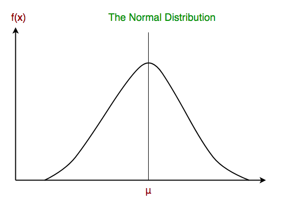
Updated table of prior probabilities for outlook feature is as following:
The likelihood of the features is assumed to be Gaussian, hence, conditional probability is given by:
[Tex] P(x_i | y) = \frac{1}{\sqrt{2\pi\sigma _{y}^{2} }} exp \left (-\frac{(x_i-\mu _{y})^2}{2\sigma _{y}^{2}} \right )
[/Tex]
Now, we look at an implementation of Gaussian Naive Bayes classifier using scikit-learn.
| Yes
| No
| P(Yes)
| P(No)
|
|---|
Sunny
|
3
|
2
|
3/9
|
2/5
|
|---|
Rainy
|
4
|
0
|
4/9
|
0/5
|
|---|
Overcast
|
2
|
3
|
2/9
|
3/5
|
|---|
Total
|
9
|
5
|
100%
|
100%
|
|---|
Python
from sklearn.datasets import load_iris
iris = load_iris()
X = iris.data
y = iris.target
from sklearn.model_selection import train_test_split
X_train, X_test, y_train, y_test = train_test_split(X, y, test_size=0.4, random_state=1)
from sklearn.naive_bayes import GaussianNB
gnb = GaussianNB()
gnb.fit(X_train, y_train)
y_pred = gnb.predict(X_test)
from sklearn import metrics
print("Gaussian Naive Bayes model accuracy(in %):", metrics.accuracy_score(y_test, y_pred)*100)
|
Output:
Gaussian Naive Bayes model accuracy(in %): 95.0
Multinomial Naive Bayes
Feature vectors represent the frequencies with which certain events have been generated by a multinomial distribution. This is the event model typically used for document classification.
Bernoulli Naive Bayes
In the multivariate Bernoulli event model, features are independent booleans (binary variables) describing inputs. Like the multinomial model, this model is popular for document classification tasks, where binary term occurrence(i.e. a word occurs in a document or not) features are used rather than term frequencies(i.e. frequency of a word in the document).
Advantages of Naive Bayes Classifier
- Easy to implement and computationally efficient.
- Effective in cases with a large number of features.
- Performs well even with limited training data.
- It performs well in the presence of categorical features.
- For numerical features data is assumed to come from normal distributions
Disadvantages of Naive Bayes Classifier
- Assumes that features are independent, which may not always hold in real-world data.
- Can be influenced by irrelevant attributes.
- May assign zero probability to unseen events, leading to poor generalization.
Applications of Naive Bayes Classifier
- Spam Email Filtering: Classifies emails as spam or non-spam based on features.
- Text Classification: Used in sentiment analysis, document categorization, and topic classification.
- Medical Diagnosis: Helps in predicting the likelihood of a disease based on symptoms.
- Credit Scoring: Evaluates creditworthiness of individuals for loan approval.
- Weather Prediction: Classifies weather conditions based on various factors.
As we reach to the end of this article, here are some important points to ponder upon:
- In spite of their apparently over-simplified assumptions, naive Bayes classifiers have worked quite well in many real-world situations, famously document classification and spam filtering. They require a small amount of training data to estimate the necessary parameters.
- Naive Bayes learners and classifiers can be extremely fast compared to more sophisticated methods. The decoupling of the class conditional feature distributions means that each distribution can be independently estimated as a one dimensional distribution. This in turn helps to alleviate problems stemming from the curse of dimensionality.
Conclusion
In conclusion, Naive Bayes classifiers, despite their simplified assumptions, prove effective in various applications, showcasing notable performance in document classification and spam filtering. Their efficiency, speed, and ability to work with limited data make them valuable in real-world scenarios, compensating for their naive independence assumption.
Frequently Asked Questions on Naive Bayes Classifiers
What is Naive Bayes real example?
Naive Bayes is a simple probabilistic classifier based on Bayes’ theorem. It assumes that the features of a given data point are independent of each other, which is often not the case in reality. However, despite this simplifying assumption, Naive Bayes has been shown to be surprisingly effective in a wide range of applications.
Why is it called Naive Bayes?
Naive Bayes is called “naive” because it assumes that the features of a data point are independent of each other. This assumption is often not true in reality, but it does make the algorithm much simpler to compute.
What is an example of a Bayes classifier?
A Bayes classifier is a type of classifier that uses Bayes’ theorem to compute the probability of a given class for a given data point. Naive Bayes is one of the most common types of Bayes classifiers.
What is better than Naive Bayes?
There are several classifiers that are better than Naive Bayes in some situations. For example, logistic regression is often more accurate than Naive Bayes, especially when the features of a data point are correlated with each other.
Can Naive Bayes probability be greater than 1?
No, the probability of an event cannot be greater than 1. The probability of an event is a number between 0 and 1, where 0 indicates that the event is impossible and 1 indicates that the event is certain.
Share your thoughts in the comments
Please Login to comment...