Grid problems involve a 2D grid of cells, often representing a map or graph. We can apply Dynamic Programming on Grids when the solution for a cell is dependent on solutions of previously traversed cells like to find a path or count number of paths or solve an optimization problem across the grid, with certain constraints on movement or cost. In this article we are going to discuss about the idea behind Dynamic Programming on Grids with their importance, use cases and some practice problems.
Idea behind Dynamic Programming (DP) on Grids:
1. Defining the state:
Each cell in the grid represents a state, characterized by its position and any relevant information (e.g., accumulated cost). Each cell is a state, uniquely identified by its coordinates (i, j). We can store additional information depending on the problem:
- For pathfinding: accumulated cost, direction of travel.
- For counting paths: number of paths reaching the cell, specific conditions met.
- For maximum/minimum value: maximum/minimum value encountered so far.
2. Defining the transition function:
This function describes how to move from one state to another, specifying the valid moves and their associated costs. This function specifies how to move between states.
- For pathfinding: define valid moves (e.g., up, down, left, right) and their associated cost (e.g., distance, penalty).
- For counting paths: enumerate all valid transitions based on problem conditions.
- For maximum/minimum value: compare current value with neighboring values and update accordingly.
3. Defining the base cases:
Define base cases to ensure that we do not move outside the grid. These are the smallest subproblems with readily known solutions:
- For pathfinding: The Starting and Ending cells often have a cost of 0.
- For counting paths: The Starting cell/row/column is initialized to 1 as boundary of the grid might have only one path reaching them.
- For maximum/minimum value: Edges might have initial specific values.
4. Iteratively filling the DP table:
Starting from the base cases, calculate the optimal solution for each state using the transition function and the solutions to its smaller subproblems.
- Start with the base cases and fill the table cell by cell.
- For each cell (i, j):
- Use the transition function to consider all valid moves from neighboring cells.
- Calculate the optimal value for the current cell based on the values of its neighbors and the transition function.
- Update the DP table with the optimal value for cell (i, j).
Importance of Dynamic Programming (DP) on Grids:
Grid problems often exhibit overlapping subproblems. This means that the optimal solution for a larger problem depends on the solutions to smaller subproblems within the grid. A naive approach would involve calculating the solutions for each cell independently, leading to significant redundancy and inefficiency. Whereas DP uses the overlapping subproblems property by storing solutions to previously encountered subproblems, significantly reducing the number of repeated calculations and leading to a more efficient solution.
Use Cases of Dynamic Programming (DP) on Grids:
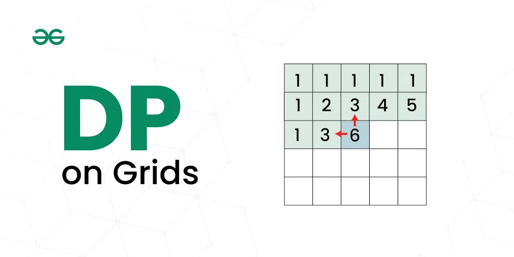
The problem is we are given a grid of size M X N and we need to count all unique possible paths from the top left to the bottom right cell with the constraints that from each cell you can either move only to the right or down. We can solve this by maintaining a 2D array count[][] of size M X N such that count[i][j] will denote the number of unique paths to reach cell (i, j) starting from (0, 0). We can initialize the first row and the first columns with all ones and then iterate over all the cells updating count[i][j] by count[i-1][j] and count[i][j-1].
The problem is we are given a grid of size M X N where some of the cells are blocked, and we need to count all unique possible paths from the top left to the bottom right cell with the constraints that from each cell you can either move only to the right or down and we can only move in the unblocked cells. We can solve this similar to the above approach and keeping track of the blocked cells and initializing the count of paths to reach the blocked cells with 0.
The problem is we are given a grid of size N X M, where ai, j = 1 denotes the cell is not empty, ai, j = 0 denotes the cell is empty, and ai, j = 2, denotes that you are standing at that cell. You can move vertically up or down and horizontally left or right to any cell which is empty. The task is to find the minimum number of steps to reach any boundary edge of the matrix. We can solve this problem by maintaining a 2D array dp[][] which stores the minimum number of steps to reach any index i, j and vis[][] to store if any particular i, j position has been visited or not previously.
The problem is we are given a cost matrix cost[][] and a position (M, N) in cost[][], find the minimum cost to reach (M, N) from (0, 0). Each cell of the matrix represents a cost to traverse through that cell. The total cost of a path to reach (M, N) is the sum of all the costs on that path (including both source and destination). You can only traverse down, right and diagonally lower cells from a given cell, i.e., from a given cell (i, j), cells (i+1, j), (i, j+1), and (i+1, j+1) can be traversed. We can solve the problem by maintaining a 2D array dp[][] such that dp[i][j] denotes the min cost to reach cell (i, j) from cell (0, 0). We can initialize the first row and column by taking the prefix sums from (0,0) to the particular cell and then iterate over the remaining cells updating dp[i][j] using dp[i-1][j], dp[i][j-1] and dp[i-1][j-1].
The problem is we are given a triangular structure of numbers, find the minimum path sum from top to bottom. Each step you may move to adjacent numbers on the row below. We can solve the problem by maintaining a 2D array dp[][] such that dp[i][j] denotes the min cost to reach cell (i, j) from the top of the triangle. We can initialize the first row and column by taking the prefix sums from (0,0) to the particular cell and then iterate over the remaining cells updating dp[i][j] using dp[i-1][j] and dp[i-1][j-1].
The problem is we are given a matrix of N * M and we have to find the maximum path sum in matrix starting from any cell in the first row and ending at any cell in the last row. The maximum path is sum of all elements from first row to last row where you are allowed to move only down or diagonally to left or right. You can start from any element in first row. The problem can be solved using a 2D array dp[][] such that dp[i][j] denotes the min cost to reach cell (i, j) from any of the cell from the first row. We can initialize the first row and column with the same value as the input matrix and then iterate over the remaining cells updating dp[i][j] using dp[i-1][j], dp[i-1][j-1] and dp[i-1][j+1].
The problem is we are given a binary matrix, and we need to find out the maximum size square sub-matrix with all 1s. The problem can be solved by using a 2D matrix dp[][] such that dp[i][j] represents the size of the square sub-matrix with all 1s including M[i][j] where M[i][j] is the rightmost and bottom-most entry in sub-matrix. We can then iterate over the cells updating dp[][] as dp[i][j] = min(dp[i][j-1], dp[i-1][j], dp[i-1][j-1]) + 1.
The problem is we are given a 2D array and we need to find the maximum sum submatrix in it. We can solve the problem in O(N^3) where we basically find top and bottom row numbers (which have maximum sum) for every fixed left and right column pair. To find the top and bottom row numbers, calculate the sum of elements in every row from left to right and store these sums in an array say temp[]. Then, we apply Kadane’s 1D algorithm on temp[], and get the maximum sum subarray of temp, this maximum sum would be the maximum possible sum with left and right as boundary columns.
The problem is we are given a matrix where every cell has some number of coins, and we have to find the count number of ways to reach bottom right from top left with exactly k coins. We can move to (i+1, j) and (i, j+1) from a cell (i, j). We can solve this by maintaining a 3D array dp[][][] such that dp[i][j][k] stores the number of ways to reach cell (i, j) starting from (0, 0) with k coins.
The problem is that we have placed two robots, one at the top left and other at the top right cell simultaneously and from a cell (i, j), the robot can move to cell (i + 1, j - 1), (i + 1, j), or (i + 1, j + 1) and we need to find the maximum number of objects the robots can collect till they reach the last row. The problem can be solved by maintaining a 3D array dp[][][], such that dp[i][j][k] stores the maximum objects collected when both the robots are in the ith row with first robot in jth column and second robot in kth column.
The problem is that we are given a 2D Matrix grid[][] of NxN size, some cells are blocked, and the remaining unblocked cells have chocolate in them. and we need to find the maximum number of chocolates that you can collect by moving from cell (0, 0) to cell (N-1, N-1) and then back to cell (0, 0). While moving from cell (0, 0) to cell (N-1, N-1), only allowed moves are: Move down (i, j) to (i+1, j) or Move Right (i, j) to (i, j+1) and while moving back from cell (N-1, N-1) to cell (0, 0), only allowed moves are: Move up (i, j) to (i-1, j) or Move left (i, j) to (i, j-1). The problem can be solved using the following approach: Instead of walking from end to beginning, let’s reverse the second leg of the path, so we can consider two persons both moving from the beginning to the end. Now, instead of considering both the paths independently we need to move both the persons simultaneously to maximize the number of chocolates. Maintain a 4D DP array dp[][][][], such that dp[r1][c1][r2][c2] stores the maximum number of chocolates we can have if the first person has reached cell (r1, c1) and the second person has reached cell(r2, c2). We can reduce the DP states to get a 3D DP array.
Practice Problems on Dynamic Programming (DP) on Grids:
Share your thoughts in the comments
Please Login to comment...