How Does Dynamic Programming Work?

Dynamic programming, popularly known as DP, is a method of solving problems by breaking them down into simple, overlapping subproblems and then solving each of the subproblems only once, storing the solutions to the subproblems that are solved to avoid redundant computations. This technique is useful for optimization-based problems, where the goal is to find the most optimal solution among all possible set of solutions.

What is Dynamic Programming?

Dynamic Programming is a problem-solving technique used to solve complex problems by breaking them into smaller overlapping subproblems and solving each subproblem only once, storing the solutions to avoid redundant computations. It often involves optimal substructure and overlapping subproblems to efficiently solve problems with recursive structures.

This approach is like the divide and conquers algorithm where a problem is divided into sub-problems and recursively solving sub-problems and combining their solution to find the solution to the original problem.

Dynamic Programming Characteristics

Dynamic programming is a way of solving tricky problems by breaking them into smaller pieces and solving each piece just once, saving the answers to avoid doing the same work over and over.

Here are two key things to check if dynamic programming is the right tool for the job:

1. Optimal Substructure:

• The problem should have optimal substructure, meaning the best solution comes from combining optimal solutions to smaller sub-problems.
• Take the Fibonacci series as an example, where the nth number is the sum of the previous two numbers: Fib(n) = Fib(n-1) + Fib(n-2).
• This shows how a problem of size “n” can be broken down into sub-problems of size “n-1” and “n-2,” helping define the base cases of the recursive algorithm (e.g., f(0) = 0, f(1) = 1).

2. Overlapping Subproblems:

• The other essential characteristic is overlapping subproblems, where the same smaller problems occur repeatedly in a recursive manner.
• By recognizing and storing the solutions to these overlapping subproblems, algorithm performance can be significantly improved.
• In the Fibonacci dynamic programming example, the tree representation reveals that sub-problems like fib(4), fib(3), fib(2), etc., appear multiple times.
• Remember, for a problem to be a good fit for dynamic programming, it needs both optimal substructure and overlapping subproblems.

Techniques to solve Dynamic Programming Problems:

1. Top-Down(Memoization):

Break down the given problem in order to begin solving it. If you see that the problem has already been solved, return the saved answer. If it hasn’t been solved, solve it and save it. This is usually easy to think of and very intuitive, This is referred to as Memoization.

2. Bottom-Up(Dynamic Programming):

Analyze the problem and see in what order the subproblems are solved, and work your way up from the trivial subproblem to the given problem. This process ensures that the subproblems are solved before the main problem. This is referred to as Bottom-up Dynamic Programming.

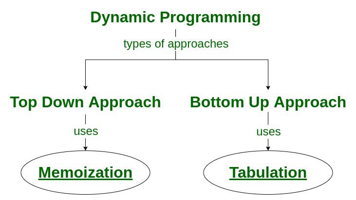
Types of the approach of dynamic programming algorithm

Understanding Dynamic Programming With Examples:

Problem: Let’s find the Fibonacci sequence up to the nth term. A Fibonacci series is the sequence of numbers in which each number is the sum of the two preceding ones. For example, 0, 1, 1, 2, 3, and so on. Here, each number is the sum of the two preceding numbers.

Naive Approach: The basic way to find the nth Fibonacci number is to use recursion.

Below is the implementation for the above approach:

C++

// C++ code for the above approach:
#include <iostream>
using namespace std;

// Function to find nth fibonacci number
int fib(int n)
{
    if (n <= 1) {
        return n;
    }
    int x = fib(n - 1);
    int y = fib(n - 2);

    return x + y;
}

// Drivers code
int main()
{
    int n = 5;

    // Function Call
    cout << fib(n);
    return 0;
}

Java

// Java code for the above approach:
import java.io.*;

class GFG {
    // Function to find nth fibonacci number
    public static int fib(int n)
    {
        if (n <= 1) {
            return n;
        }
        int x = fib(n - 1);
        int y = fib(n - 2);

        return x + y;
    }

    // Driver Code
    public static void main(String[] args)
    {
        int n = 5;

        // Function Call
        System.out.print(fib(n));
    }
}

// This code is contributed by Rohit Pradhan

Python

# Function to find nth fibonacci number
def fib(n):
    if (n <= 1):
        return n
    x = fib(n - 1)
    y = fib(n - 2)

    return x + y

n = 5;

# Function Call
print(fib(n))

#contributed by akashish__

C#

using System;

public class GFG {

    // Function to find nth fibonacci number
    public static int fib(int n)
    {
        if (n <= 1) {
            return n;
        }
        int x = fib(n - 1);
        int y = fib(n - 2);

        return x + y;
    }

    static public void Main()
    {

        int n = 5;

        // Function Call
        Console.WriteLine(fib(n));
    }
}
// contributed by akashish__

Javascript

// Function to find nth fibonacci number
function fib(n)
{
    if (n <= 1) {
        return n;
    }
    let x = fib(n - 1);
    let y = fib(n - 2);

    return x + y;
}

// Drivers code
let n = 5;

// Function Call
console.log(fib(n));

// This code is contributed by akashish__

Output

5

Complexity Analysis:

• Time Complexity: O(2ⁿ)
  • Here, for every n, we are required to make a recursive call to fib(n – 1) and fib(n – 2). For fib(n – 1), we will again make the recursive call to fib(n – 2) and fib(n – 3). Similarly, for fib(n – 2), recursive calls are made on fib(n – 3) and fib(n – 4) until we reach the base case.
  • During each recursive call, we perform constant work(k) (adding previous outputs to obtain the current output). We perform 2nK work at every level (where n = 0, 1, 2, …). Since n is the number of calls needed to reach 1, we are performing 2n-1k at the final level. Total work can be calculated as:
  • If we draw the recursion tree of the Fibonacci recursion then we found the maximum height of the tree will be n and hence the space complexity of the Fibonacci recursion will be O(n).

Efficient approach: As it is a very terrible complexity(Exponential), thus we need to optimize it with an efficient method. (Memoization)

Let’s look at the example below for finding the 5th Fibonacci number.

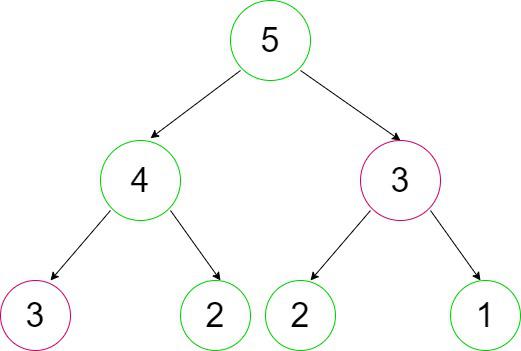
Observations:

• The entire program repeats recursive calls. As in the above figure, for calculating fib(4), we need the value of fib(3) (first recursive call over fib(3)), and for calculating fib(5), we again need the value of fib(3)(second similar recursive call over fib(3)).
• Both of these recursive calls are shown above in the outlining circle.
• Similarly, there are many others for which we are repeating the recursive calls.
• Recursion generally involves repeated recursive calls, which increases the program’s time complexity.
• By storing the output of previously encountered values (preferably in arrays, as these can be traversed and extracted most efficiently), we can overcome this problem. The next time we make a recursive call over these values, we will use their already stored outputs instead of calculating them all over again.
• In this way, we can improve the performance of our code. Memoization is the process of storing each recursive call’s output for later use, preventing the code from calculating it again.
• Way to memoize: To achieve this in our example we will simply take an answer array initialized to -1. As we make a recursive call, we will first check if the value stored in the answer array corresponding to that position is -1. The value -1 indicates that we haven’t calculated it yet and have to recursively compute it. The output must be stored in the answer array so that, next time, if the same value is encountered, it can be directly used from the answer array.
• Now in this process of memoization, considering the above Fibonacci numbers example, it can be observed that the total number of unique calls will be at most (n + 1) only.

Below is the implementation for the above approach:

C++

// C++ code for the above approach:
#include <iostream>
using namespace std;

// Helper Function
int fibo_helper(int n, int* ans)
{

    // Base case
    if (n <= 1) {
        return n;
    }

    // To check if output already exists
    if (ans[n] != -1) {
        return ans[n];
    }

    // Calculate output
    int x = fibo_helper(n - 1, ans);
    int y = fibo_helper(n - 2, ans);

    // Saving the output for future use
    ans[n] = x + y;

    // Returning the final output
    return ans[n];
}

int fibo(int n)
{
    int* ans = new int[n + 1];

    // Initializing with -1
    for (int i = 0; i <= n; i++) {
        ans[i] = -1;
    }
    fibo_helper(n, ans);
}

// Drivers code
int main()
{
    int n = 5;

    // Function Call
    cout << fibo(n);
    return 0;
}

Java

// Java code for the above approach:
import java.io.*;

class GFG {
    // Helper Function
    public static int fibo_helper(int n, int ans[])
    {

        // Base case
        if (n <= 1) {
            return n;
        }

        // To check if output already exists
        if (ans[n] != -1) {
            return ans[n];
        }

        // Calculate output
        int x = fibo_helper(n - 1, ans);
        int y = fibo_helper(n - 2, ans);

        // Saving the output for future use
        ans[n] = x + y;

        // Returning the final output
        return ans[n];
    }

    public static int fibo(int n)
    {
        int ans[] = new int[n + 1];

        // Initializing with -1
        for (int i = 0; i <= n; i++) {
            ans[i] = -1;
        }
        return fibo_helper(n, ans);
    }

    // Driver Code
    public static void main(String[] args)
    {
        int n = 5;

        // Function Call
        System.out.print(fibo(n));
    }
}

// This code is contributed by Rohit Pradhan

Python

# Helper Function
def fibo_helper(n, ans):


    # Base case
if (n <= 1):
    return n

# To check if output already exists
if (ans[n] is not -1):
    return ans[n]

# Calculate output
x = fibo_helper(n - 1, ans)
y = fibo_helper(n - 2, ans)

# Saving the output for future use
ans[n] = x + y

# Returning the final output
return ans[n]


def fibo(n):


ans = [-1]*(n+1)

# Initializing with -1
# for (i = 0; i <= n; i++) {
for i in range(0, n+1):
    ans[i] = -1

return fibo_helper(n, ans)


# Code
n = 5

# Function Call
print(fibo(n))
# contributed by akashish__

C#

using System;

public class GFG {

    // Helper Function
    public static int fibo_helper(int n, int[] ans)
    {

        // Base case
        if (n <= 1) {
            return n;
        }

        // To check if output already exists
        if (ans[n] != -1) {
            return ans[n];
        }

        // Calculate output
        int x = fibo_helper(n - 1, ans);
        int y = fibo_helper(n - 2, ans);

        // Saving the output for future use
        ans[n] = x + y;

        // Returning the final output
        return ans[n];
    }

    public static int fibo(int n)
    {
        int[] ans = new int[n + 1];

        // Initializing with -1
        for (int i = 0; i <= n; i++) {
            ans[i] = -1;
        }
        return fibo_helper(n, ans);
    }

    static public void Main()
    {

        // Code

        int n = 5;

        // Function Call
        Console.WriteLine(fibo(n));
    }
}
// contributed by akashish__

Javascript

<script>

// Javascript code for the above approach:

// Helper Function
function fibo_helper(n, ans) {
    // Base case
    if (n <= 1) {
        return n;
    }

    // To check if output already exists
    if (ans[n] != -1) {
        return ans[n];
    }

    // Calculate output
    let x = fibo_helper(n - 1, ans);
    let y = fibo_helper(n - 2, ans);

    // Saving the output for future use
    ans[n] = x + y;

    // Returning the final output
    return ans[n];
}

function fibo(n) {
    let ans = [];

    // Initializing with -1
    for (let i = 0; i <= n; i++) {
        ans.push(-1);
    }
    return fibo_helper(n, ans);
}

// Drivers code
let n = 5;

// Function Call
console.log(fibo(n));

// contributed by akashish__

</script>

Output

5

Time complexity: O(n)
Auxiliary Space: O(n)

Optimized approach: Following a bottom-up approach to reach the desired index. This approach of converting recursion into iteration is known as Bottom up-Dynamic programming(DP).

Observations:

• Finally, what we do is recursively call each response index field and calculate its value using previously saved outputs.
• Recursive calls terminate via the base case, which means we are already aware of the answers which should be stored in the base case indexes.
• In the case of Fibonacci numbers, these indices are 0 and 1 as f(ib0) = 0 and f(ib1) = 1. So we can directly assign these two values ​​into our answer array and then use them to calculate f(ib2), which is f(ib1) + f(ib0), and so on for each subsequent index.
• This can easily be done iteratively by running a loop from i = (2 to n). Finally, we get our answer at the 5th index of the array because we already know that the ith index contains the answer to the ith value.
• Simply, we first try to find out the dependence of the current value on previous values ​​and then use them to calculate our new value. Now, we are looking for those values which do not depend on other values, which means they are independent(base case values, since these, are the smallest problems
• which we are already aware of).

Below is the implementation for the above approach:

C++

// C++ code for the above approach:
#include <iostream>
using namespace std;

// Helper Function
int fibo_helper(int n, int* ans)
{

    // Base case
    if (n <= 1) {
        return n;
    }

    // To check if output already exists
    if (ans[n] != -1) {
        return ans[n];
    }

    // Calculate output
    int x = fibo_helper(n - 1, ans);
    int y = fibo_helper(n - 2, ans);

    // Saving the output for future use
    ans[n] = x + y;

    // Returning the final output
    return ans[n];
}

int fibo(int n)
{
    int* ans = new int[n + 1];

    // Initializing with -1
    for (int i = 0; i <= n; i++) {
        ans[i] = -1;
    }
    fibo_helper(n, ans);
}

// Drivers code
int main()
{
    int n = 5;

    // Function Call
    cout << fibo(n);
    return 0;
}

Java

// Java code for the above approach:
import java.io.*;

class GFG {
    // Function for calculating the nth
    // Fibonacci number
    public static int fibo(int n)
    {
        int ans[] = new int[n + 1];

        // Storing the independent values in the
        // answer array
        ans[0] = 0;
        ans[1] = 1;

        // Using the bottom-up approach
        for (int i = 2; i <= n; i++) {
            ans[i] = ans[i - 1] + ans[i - 2];
        }

        // Returning the final index
        return ans[n];
    }

    // Driver Code
    public static void main(String[] args)
    {
        int n = 5;

        // Function Call
        System.out.print(fibo(n));
    }
}

// This code is contributed by Rohit Pradhan

Python

# Python3 code for the above approach:

# Function for calculating the nth
# Fibonacci number
def fibo(n):
ans = [None] * (n + 1)

# Storing the independent values in the
# answer array
ans[0] = 0
ans[1] = 1

# Using the bottom-up approach
for i in range(2,n+1):
    ans[i] = ans[i - 1] + ans[i - 2]

# Returning the final index
return ans[n]

# Drivers code
n = 5

# Function Call
print(fibo(n))
#contributed by akashish__

C#

// C# code for the above approach:

using System;

public class GFG {

    // Function for calculating the nth
    // Fibonacci number
    public static int fibo(int n)
    {
        int[] ans = new int[n + 1];

        // Storing the independent values in the
        // answer array
        ans[0] = 0;
        ans[1] = 1;

        // Using the bottom-up approach
        for (int i = 2; i <= n; i++) {
            ans[i] = ans[i - 1] + ans[i - 2];
        }

        // Returning the final index
        return ans[n];
    }

    static public void Main()
    {

        // Code
        int n = 5;

        // Function Call
        Console.Write(fibo(n));
    }
}

// This code is contributed by lokeshmvs21.

Javascript

// Function for calculating the nth Fibonacci number
function fibo(n) {
    // Array to store Fibonacci numbers
    let ans = new Array(n + 1);

    // Storing the initial Fibonacci values
    ans[0] = 0;
    ans[1] = 1;

    // Using the bottom-up approach to calculate Fibonacci numbers
    for (let i = 2; i <= n; i++) {
        ans[i] = ans[i - 1] + ans[i - 2];
    }

    // Returning the nth Fibonacci number
    return ans[n];
}

// Driver code
function main() {
    let n = 5;

    // Function call
    console.log(fibo(n));
}

// Calling the main function to execute the program
main();

// This code is contributed by shivamgupta310570

Output

5

Time complexity: O(n)
Auxiliary Space: O(n)

Conclusion

Dynamic programming, also known as DP, is a problem-solving technique that is very powerful. It breaks complex problems into simpler, overlapping subproblems and then, one by one, solves each problem. Memorization and tabulation are two approaches to implementing dynamic programming. Memorization, a top-bottom approach, optimises recursive solutions by storing results in a memo table. Tabulation, a bottom-up approach, builds solutions through an iterative approach and provides an efficient alternative. Both techniques enhance algorithm efficiency, as demonstrated in the Fibonacci numbers example, optimizing time and space complexities.