ML | Stochastic Gradient Descent (SGD)

Gradient Descent is an iterative optimization process that searches for an objective function’s optimum value (Minimum/Maximum). It is one of the most used methods for changing a model’s parameters in order to reduce a cost function in machine learning projects.  

The primary goal of gradient descent is to identify the model parameters that provide the maximum accuracy on both training and test datasets. In gradient descent, the gradient is a vector pointing in the general direction of the function’s steepest rise at a particular point. The algorithm might gradually drop towards lower values of the function by moving in the opposite direction of the gradient, until reaching the minimum of the function.

Types of Gradient Descent: 

Typically, there are three types of Gradient Descent:  

1. Batch Gradient Descent
2. Stochastic Gradient Descent
3. Mini-batch Gradient Descent

In this article, we will be discussing Stochastic Gradient Descent (SGD). 

Stochastic Gradient Descent (SGD):

Stochastic Gradient Descent (SGD) is a variant of the Gradient Descent algorithm that is used for optimizing machine learning models. It addresses the computational inefficiency of traditional Gradient Descent methods when dealing with large datasets in machine learning projects.

In SGD, instead of using the entire dataset for each iteration, only a single random training example (or a small batch) is selected to calculate the gradient and update the model parameters. This random selection introduces randomness into the optimization process, hence the term “stochastic” in stochastic Gradient Descent

The advantage of using SGD is its computational efficiency, especially when dealing with large datasets. By using a single example or a small batch, the computational cost per iteration is significantly reduced compared to traditional Gradient Descent methods that require processing the entire dataset.

Stochastic Gradient Descent Algorithm 

• Initialization: Randomly initialize the parameters of the model.
• Set Parameters: Determine the number of iterations and the learning rate (alpha) for updating the parameters.
• Stochastic Gradient Descent Loop: Repeat the following steps until the model converges or reaches the maximum number of iterations: 
  • Shuffle the training dataset to introduce randomness. 
  • Iterate over each training example (or a small batch) in the shuffled order. 
  • Compute the gradient of the cost function with respect to the model parameters using the current training
    example (or batch).
  • Update the model parameters by taking a step in the direction of the negative gradient, scaled by the learning rate. 
  • Evaluate the convergence criteria, such as the difference in the cost function between iterations of the gradient.
• Return Optimized Parameters: Once the convergence criteria are met or the maximum number of iterations is reached, return the optimized model parameters.

In SGD, since only one sample from the dataset is chosen at random for each iteration, the path taken by the algorithm to reach the minima is usually noisier than your typical Gradient Descent algorithm. But that doesn’t matter all that much because the path taken by the algorithm does not matter, as long as we reach the minimum and with a significantly shorter training time.

The path taken by Batch Gradient Descent is shown below:

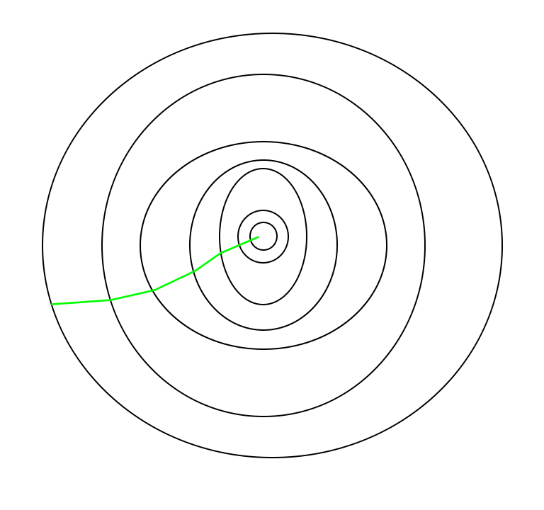
Batch gradient optimization path 

A path taken by Stochastic Gradient Descent looks as follows –  

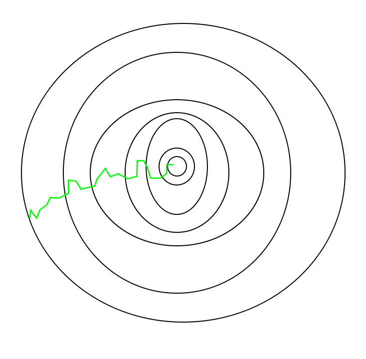
stochastic gradient optimization path 

One thing to be noted is that, as SGD is generally noisier than typical Gradient Descent, it usually took a higher number of iterations to reach the minima, because of the randomness in its descent. Even though it requires a higher number of iterations to reach the minima than typical Gradient Descent, it is still computationally much less expensive than typical Gradient Descent. Hence, in most scenarios, SGD is preferred over Batch Gradient Descent for optimizing a learning algorithm.

Difference between Stochastic Gradient Descent & batch Gradient Descent 

The comparison between Stochastic Gradient Descent (SGD) and Batch Gradient Descent are as follows:

Aspect	Stochastic Gradient Descent (SGD)	Batch Gradient Descent
Dataset Usage	Uses a single random sample or a small batch of samples at each iteration.	Uses the entire dataset (batch) at each iteration.
Computational Efficiency	Computationally less expensive per iteration, as it processes fewer data points.	Computationally more expensive per iteration, as it processes the entire dataset.
Convergence	Faster convergence due to frequent updates.	Slower convergence due to less frequent updates.
Noise in Updates	High noise due to frequent updates with a single or few samples.	Low noise as it updates parameters using all data points.
Stability	Less stable as it may oscillate around the optimal solution.	More stable as it converges smoothly towards the optimum.
Memory Requirement	Requires less memory as it processes fewer data points at a time.	Requires more memory to hold the entire dataset in memory.
Update Frequency	Frequent updates make it suitable for online learning and large datasets.	Less frequent updates make it suitable for smaller datasets.
Initialization Sensitivity	Less sensitive to initial parameter values due to frequent updates.	More sensitive to initial parameter values.

Python Code For Stochastic Gradient Descent 

We will create an SGD class with methods that we will use while updating the parameters, fitting the training data set, and predicting the new test data. The methods we will be using are as :

1. The first line imports the NumPy library, which is used for numerical computations in Python.
2. Define the SGD class:
   1. The class SGD encapsulates the Stochastic Gradient Descent algorithm for training a linear regression model.
   2. Then we initialize the SGD optimizer parameters such as learning rate, number of epochs, batch size, and tolerance. It also initializes weights and bias to None.
   3. predict function: This function computes the predictions for input data X using the current weights and bias. It performs matrix multiplication between input X and weights, and then adds the bias term.
   4. mean_squared_error function: This function calculates the mean squared error between the true target values y_true and the predicted values y_pred.
   5. gradient function: This computes the gradients of the loss function with respect to the weights and bias using the formula for the gradient of the mean squared error loss function.
   6. fit method: This method fits the model to the training data using stochastic gradient descent. It iterates through the specified number of epochs, shuffling the data and updating the weights and bias in each epoch. It also prints the loss periodically and checks for convergence based on the tolerance.
      1. it calculates gradients using a mini-batch of data (X_batch, y_batch). This aligns with the stochastic nature of SGD.
      2. After computing the gradients, the method updates the model parameters (self.weights and self.bias) using the learning rate and the calculated gradients. This is consistent with the parameter update step in SGD.
      3. The fit method iterates through the entire dataset (X, y) for each epoch. However, it updates the parameters using mini-batches, as indicated by the nested loop that iterates through the dataset in mini-batches (for i in range(0, n_samples, self.batch_size)). This reflects the stochastic nature of SGD, where parameters are updated using a subset of the data.

Python3

import numpy as np

class SGD:
    def __init__(self, lr=0.01, epochs=1000, batch_size=32, tol=1e-3):
        self.learning_rate = lr
        self.epochs = epochs
        self.batch_size = batch_size
        self.tolerance = tol
        self.weights = None
        self.bias = None

    def predict(self, X):
        return np.dot(X, self.weights) + self.bias

    def mean_squared_error(self, y_true, y_pred):
        return np.mean((y_true - y_pred) ** 2)

    def gradient(self, X_batch, y_batch):
        y_pred = self.predict(X_batch)
        error = y_pred - y_batch
        gradient_weights = np.dot(X_batch.T, error) / X_batch.shape[0]
        gradient_bias = np.mean(error)
        return gradient_weights, gradient_bias

    def fit(self, X, y):
        n_samples, n_features = X.shape
        self.weights = np.random.randn(n_features)
        self.bias = np.random.randn()

        for epoch in range(self.epochs):
            indices = np.random.permutation(n_samples)
            X_shuffled = X[indices]
            y_shuffled = y[indices]

            for i in range(0, n_samples, self.batch_size):
                X_batch = X_shuffled[i:i+self.batch_size]
                y_batch = y_shuffled[i:i+self.batch_size]

                gradient_weights, gradient_bias = self.gradient(X_batch, y_batch)
                self.weights -= self.learning_rate * gradient_weights
                self.bias -= self.learning_rate * gradient_bias

            if epoch % 100 == 0:
                y_pred = self.predict(X)
                loss = self.mean_squared_error(y, y_pred)
                print(f"Epoch {epoch}: Loss {loss}")

            if np.linalg.norm(gradient_weights) < self.tolerance:
                print("Convergence reached.")
                break

        return self.weights, self.bias

SGD Implementation 

We will create a random dataset with 100 rows and 5 columns and we fit our Stochastic gradient descent Class on this data.  Also, We will use predict method from SGD

Python3

# Create random dataset with 100 rows and 5 columns
X = np.random.randn(100, 5)
# create corresponding target value by adding random
# noise in the dataset
y = np.dot(X, np.array([1, 2, 3, 4, 5]))\
    + np.random.randn(100) * 0.1
# Create an instance of the SGD class
model = SGD(lr=0.01, epochs=1000,
            batch_size=32, tol=1e-3)
w,b=model.fit(X,y)
# Predict using predict method from model
y_pred = w*X+b
#y_pred

Output:

Epoch 0: Loss 64.66196845798673
Epoch 100: Loss 0.03999940087439455
Epoch 200: Loss 0.008260358272771882
Epoch 300: Loss 0.00823731979566282
Epoch 400: Loss 0.008243022613956992
Epoch 500: Loss 0.008239370268212335
Epoch 600: Loss 0.008236363304624746
Epoch 700: Loss 0.00823205131002819
Epoch 800: Loss 0.00823566681302786
Epoch 900: Loss 0.008237441485197143

This cycle of taking the values and adjusting them based on different parameters in order to reduce the loss function is called back-propagation.

Stochastic Gradient Descent (SGD) using TensorFLow

we can apply the above code using the TensorFLow.

Python3

import tensorflow as tf
import numpy as np

class SGD:
    def __init__(self, lr=0.001, epochs=2000, batch_size=32, tol=1e-3):
        self.learning_rate = lr
        self.epochs = epochs
        self.batch_size = batch_size
        self.tolerance = tol
        self.weights = None
        self.bias = None

    def predict(self, X):
        return tf.matmul(X, self.weights) + self.bias

    def mean_squared_error(self, y_true, y_pred):
        return tf.reduce_mean(tf.square(y_true - y_pred))

    def gradient(self, X_batch, y_batch):
        with tf.GradientTape() as tape:
            y_pred = self.predict(X_batch)
            loss = self.mean_squared_error(y_batch, y_pred)
        gradient_weights, gradient_bias = tape.gradient(loss, [self.weights, self.bias])
        return gradient_weights, gradient_bias

    def fit(self, X, y):
        n_samples, n_features = X.shape
        self.weights = tf.Variable(tf.random.normal((n_features, 1)))
        self.bias = tf.Variable(tf.random.normal(()))

        for epoch in range(self.epochs):
            indices = tf.random.shuffle(tf.range(n_samples))
            X_shuffled = tf.gather(X, indices)
            y_shuffled = tf.gather(y, indices)

            for i in range(0, n_samples, self.batch_size):
                X_batch = X_shuffled[i:i+self.batch_size]
                y_batch = y_shuffled[i:i+self.batch_size]

                gradient_weights, gradient_bias = self.gradient(X_batch, y_batch)
                # Gradient clipping
                gradient_weights = tf.clip_by_value(gradient_weights, -1, 1)
                gradient_bias = tf.clip_by_value(gradient_bias, -1, 1)
                
                self.weights.assign_sub(self.learning_rate * gradient_weights)
                self.bias.assign_sub(self.learning_rate * gradient_bias)

            if epoch % 100 == 0:
                y_pred = self.predict(X)
                loss = self.mean_squared_error(y, y_pred)
                print(f"Epoch {epoch}: Loss {loss}")

            if tf.norm(gradient_weights) < self.tolerance:
                print("Convergence reached.")
                break

        return self.weights.numpy(), self.bias.numpy()

# Create random dataset with 100 rows and 5 columns
X = np.random.randn(100, 5).astype(np.float32)
# Create corresponding target value by adding random
# noise in the dataset
y = np.dot(X, np.array([1, 2, 3, 4, 5], dtype=np.float32)) + np.random.randn(100).astype(np.float32) * 0.1

# Create an instance of the SGD class
model = SGD(lr=0.005, epochs=1000, batch_size=12, tol=1e-3)
w, b = model.fit(X, y)

# Predict using predict method from model
y_pred = np.dot(X, w) + b

Output:

Epoch 0: Loss 52.73115158081055
Epoch 100: Loss 44.69907760620117
Epoch 200: Loss 44.693603515625
Epoch 300: Loss 44.69377136230469
Epoch 400: Loss 44.67509460449219
Epoch 500: Loss 44.67082595825195
Epoch 600: Loss 44.674285888671875
Epoch 700: Loss 44.666194915771484
Epoch 800: Loss 44.66718292236328
Epoch 900: Loss 44.65559005737305

Advantages of Stochastic Gradient Descent  

• Speed: SGD is faster than other variants of Gradient Descent such as Batch Gradient Descent and Mini-Batch Gradient Descent since it uses only one example to update the parameters.
• Memory Efficiency: Since SGD updates the parameters for each training example one at a time, it is memory-efficient and can handle large datasets that cannot fit into memory.
• Avoidance of Local Minima: Due to the noisy updates in SGD, it has the ability to escape from local minima and converges to a global minimum.

Disadvantages of Stochastic Gradient Descent 

• Noisy updates: The updates in SGD are noisy and have a high variance, which can make the optimization process less stable and lead to oscillations around the minimum.
• Slow Convergence: SGD may require more iterations to converge to the minimum since it updates the parameters for each training example one at a time.
• Sensitivity to Learning Rate: The choice of learning rate can be critical in SGD since using a high learning rate can cause the algorithm to overshoot the minimum, while a low learning rate can make the algorithm converge slowly.
• Less Accurate: Due to the noisy updates, SGD may not converge to the exact global minimum and can result in a suboptimal solution. This can be mitigated by using techniques such as learning rate scheduling and momentum-based updates.