Classification on Imbalanced data using Tensorflow

In the modern days of machine learning, imbalanced datasets are like a curse that degrades the overall model performance in classification tasks. In this article, we will implement a Deep learning model using TensorFlow for classification on a highly imbalanced dataset.

Classification on Imbalanced data using Tensorflow

What is Imbalanced Data?

Most real-world datasets are imbalanced. A dataset can be called imbalanced when the distribution of classes of the target variable of the dataset is highly skewed i.e. the occurrence of one class (minority class) is significantly low from the majority class. This imbalanced dataset greatly reduces the model’s performance, degrades the learning process and induces biasing within the model’s prediction which leads to wrong and suboptimal predictions. In practical terms, consider a medical diagnosis model attempting to identify a rare disease—where positive cases are sparse compared to negatives. The skewed distribution can potentially compromise the model’s ability to generalize and make accurate predictions. So, it is very important to handle imbalanced datasets carefully to achieve optimal model performance.

Step-by-Step Code Implementations

Importing required libraries

At first, we will import all required Python libraries like NumPy, Pandas, Matplotlib, Seaborn, TensorFlow, SKlearn etc.

Python3

import numpy as np
import pandas as pd
import matplotlib.pyplot as plt
import seaborn as sns
from sklearn.preprocessing import MinMaxScaler, LabelEncoder
from sklearn.model_selection import train_test_split
from sklearn.metrics import accuracy_score, precision_score, recall_score, f1_score
import tensorflow as tf
from tensorflow.keras.models import Sequential
from tensorflow.keras.layers import Dense

Dataset loading

Before loading the dataset, we will handle the randomness of the runtime resources using random seeding. After that, we will load a dataset. Then we will perform simple outlier removal so that our final results are not getting biased.

Python3

# Set random seed for reproducibility
seed = 42
np.random.seed(seed)
tf.random.set_seed(seed)
# Set random seed for reproducibility on GPU
tf.config.experimental.set_visible_devices([], 'GPU')
# load the dataset
df = pd.read_csv("data.csv") # https://www.kaggle.com/datasets/uciml/breast-cancer-wisconsin-data/data?select=data.csv
df.drop(columns=['id', 'Unnamed: 32'], inplace=True)

# Outlier removal
numerical_columns = df.select_dtypes(exclude=object).columns.tolist()

for col in numerical_columns:
    upper_limit = df[col].mean() + 3 * df[col].std()
    lower_limit = df[col].mean() - 3 * df[col].std()
    df = df[(df[col] <= upper_limit) & (df[col] >= lower_limit)]

Data pre-processing and splitting

Now we will scale numerical columns of the dataset using MinMaxScaler and the target column will be encoded by Label encoder. Then the dataset will be divided into training and testing sets(80:20).

Python3

# Scaling The Numerical Columns Using The MinMax Scaler
scaler = MinMaxScaler()
df[numerical_columns] = scaler.fit_transform(df[numerical_columns])
# Encoding The Target Column Using Label Encoder
encoder = LabelEncoder()
df['diagnosis'] = encoder.fit_transform(df['diagnosis'])
# data spliting
X = df.drop(columns=['diagnosis'])
y = df['diagnosis']
X_train, X_test, y_train, y_test = train_test_split(X, y, test_size=0.2, random_state=42)

Check for imbalance

We are performing classification of imbalance dataset. So, it required see how the target column is distributed. This Exploratory Data Analysis will help to under that imbalance factor of the dataset.

Python3

# Visualize the distribution of the target variable in a pie chart
plt.figure(figsize=(6, 6))
df['diagnosis'].value_counts().plot(kind='pie', autopct='%1.1f%%', colors=['skyblue', 'lightcoral'])
plt.title('Distribution of Diagnosis (Malignant vs Benign)')
plt.ylabel('')
plt.show()

Output:

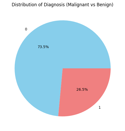
Distribution of target column

So, we can say that the dataset is highly imbalanced as there is a difference of approximately 3X of occurrences between ‘Malignant’ and ‘Benign’ classes. Now we can smoothly proceed with this dataset.

Class weights calculation

As we are performing classification on imbalance dataset so it is required to manually calculate the class weights for both majority and minority classes. This class weights will be stored in a variable and directed feed to the model during training.

Python3

# Calculate class weights
total = len(y_train)
pos = np.sum(y_train == 1)
neg = np.sum(y_train == 0)

weight_for_0 = (1 / neg) * (total / 2.0)
weight_for_1 = (1 / pos) * (total / 2.0)

class_weight = {0: weight_for_0, 1: weight_for_1}

print('Weight for class 0: {:.2f}'.format(weight_for_0))
print('Weight for class 1: {:.2f}'.format(weight_for_1))

Output:

Weight for class 0: 0.68
Weight for class 1: 1.87

Defining the Deep Leaning model

Now we will define our three-layered Deep Learning model and we will use loss as ‘binary_crossentropy’ which is used for binary classification and optimizer as ‘adam’.

Python3

model = Sequential([
    Dense(16, activation='relu', input_dim=30),
    Dense(8, activation='relu'),
    Dense(1, activation='sigmoid')
])

model.compile(optimizer='adam', loss='binary_crossentropy', metrics=['accuracy'])
model.summary()

Output:

  Model: "sequential"
_________________________________________________________________
 Layer (type)                Output Shape              Param #   
=================================================================
 dense (Dense)               (None, 16)                496       
                                                                 
 dense_1 (Dense)             (None, 8)                 136       
                                                                 
 dense_2 (Dense)             (None, 1)                 9         
                                                                 
=================================================================
Total params: 641 (2.50 KB)
Trainable params: 641 (2.50 KB)
Non-trainable params: 0 (0.00 Byte)
_________________________________________________________________

Model training

We are all set up for model training. We will train the model on 80 epochs. However, it is suggested that more epochs will give better results. Also, here we need to pass a hyper-parameter called class_weight. This can be decided by the formula which is: , where is class weight, N is total samples, is total number of classes and is corresponding class samples.

Python3

history = model.fit(X_train, y_train, epochs=80, validation_data=(X_test, y_test), class_weight=class_weight)

Output:

Epoch 1/80
11/11 [==============================] - 1s 25ms/step - loss: 0.6723 - accuracy: 0.6686 - val_loss: 0.6508 - val_accuracy: 0.7442
.......................................
.......................................
Epoch 80/80
11/11 [==============================] - 0s 5ms/step - loss: 0.0729 - accuracy: 0.9677 - val_loss: 0.1415 - val_accuracy: 0.9419

As the output is large so we are only giving the initial and last epoch for understanding.

Visualizing the training process

For better understanding how our model is learning and progressing at each epoch, we will plot the loss vs. accuracy curve.

Python3

# Plot Loss vs. Accuracy
plt.figure(figsize=(10, 4))

# Plot Training vs. validation Loss
plt.subplot(1, 2, 1)
plt.plot(history.history['loss'], label='Training Loss')
plt.plot(history.history['val_loss'], label='Validation Loss')
plt.title('Training vs. Validation Loss')
plt.xlabel('Epochs')
plt.ylabel('Loss')
plt.legend()

# Plot Training vs. validation Accuracy
plt.subplot(1, 2, 2)
plt.plot(history.history['accuracy'], label='Training Accuracy')
plt.plot(history.history['val_accuracy'], label='Validation Accuracy')
plt.title('Training vs. Validation Accuracy')
plt.xlabel('Epochs')
plt.ylabel('Accuracy')
plt.legend()

plt.tight_layout()
plt.show()

Output:

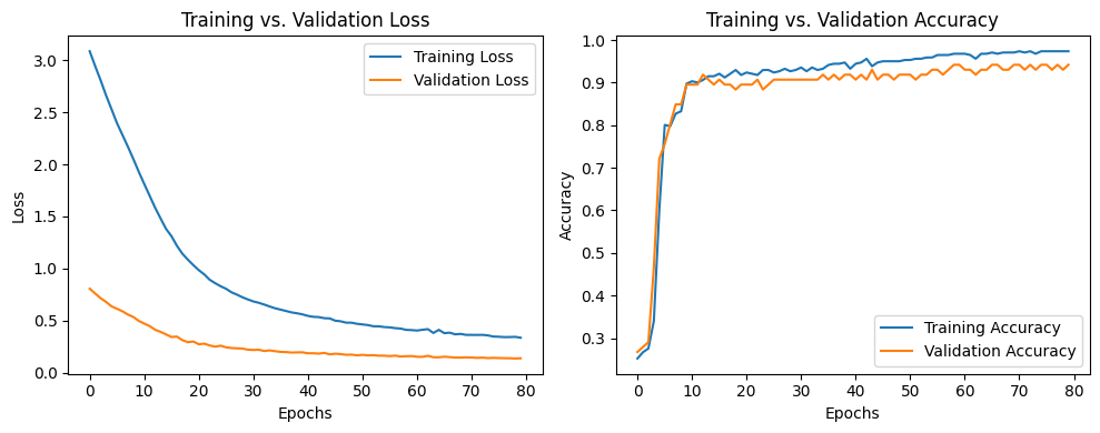
Loss vs. Accuracy curve

The above plot clearly depicts that more we go forward with epochs, our model will learn better. So, it is suggested that for better results go for more epochs.

Setting best Bias factor

To evaluate our model, we need to set the bias factor. It is basically a value which indicates the borderline of majority and minority class outputs. Now we can set by assumption but it will be good if we set it by tuning. We will perform tuning based on best F1-score and use that value further.

Python3

y_pred = model.predict(X_test)
biasing = np.arange(0.4, 0.9)   # range 40% to 90% bias
f1_scores = [] # bias setting based on best f1-score

for bias in biasing:
    y_pred_binary = (y_pred > bias).astype(int)
    f1 = f1_score(y_test, y_pred_binary)
    f1_scores.append(f1)

best_bias = biasing[np.argmax(f1_scores)]
print("Best Bias:", best_bias)

Output:

 3/3 [==============================] - 0s 3ms/step
Best Bias: 0.4

Model Evaluation

For binary classification on imbalanced dataset Accuracy is not enough for evaluation. Besides Accuracy, we will evaluate our model in the terms of Precision, Recall and F1-Score. Here we need to set the bias.

Python3

import sklearn
print(sklearn.metrics.classification_report(y_test, y_pred_binary))

Output:

              precision    recall  f1-score   support

           0       0.97      0.92      0.94        64
           1       0.80      0.91      0.85        22

    accuracy                           0.92        86
   macro avg       0.88      0.92      0.90        86
weighted avg       0.92      0.92      0.92        86

Confusion matrix

Now let us visualize the confusion matrix. It will help us to analyze the predictions with actual.

Python3

# Create a confusion matrix
cm = confusion_matrix(y_test, y_pred_binary)

# Plot the colorful confusion matrix
plt.figure(figsize=(4, 3))
sns.heatmap(cm, annot=True, fmt='d', cmap='Blues', xticklabels=['Benign', 'Malignant'], yticklabels=['Benign', 'Malignant'])
plt.title('Confusion Matrix')
plt.xlabel('Predicted')
plt.ylabel('Actual')
plt.show()

Output:

Conclusion

We can conclude that classification on imbalanced dataset is very crucial task as all real-world datasets are imbalanced in nature. Our model achieved notable 94% of accuracy and high F1-Score of 88% which denotes that the model is performing well.