3D Curve Fitting With Python

Curve fitting is a widely used technique in the field of data analysis and mathematical modeling. It involves the process of finding a mathematical function that best approximates a set of data points. In 3D curve fitting, the process is extended to three-dimensional space, where the goal is to find a function that best represents a set of 3D data points.

Python is a popular programming language used for scientific computing, and it provides several libraries that can be used for 3D curve fitting. In this article, we will discuss how to perform 3D curve fitting in Python using the SciPy library. so here In this article, we use how the SciPy library will be used for 3D curve fitting.

SciPy Library

The SciPy library is a powerful tool for scientific computing in Python. It provides a wide range of functionality for optimization, integration, interpolation, and curve fitting. In this article, we will focus on the curve-fitting capabilities of the library.

SciPy provides the curve_fit function, which can be used to perform curve fitting in Python. The function takes as input the data points to be fitted and the mathematical function to be used for fitting. The function then returns the optimized parameters for the mathematical function that best approximates the input data. 

Let’s see the full step-by-step process for doing 3D Curve Fitting of 100 randomly generated points using the SciPy library in Python.

Prerequisites Library: here we use NumPy for generating random points and storing them, SciPy, and matplotlib for plotting these points in 3D space. so first of all install them using the below command in the terminal.

pip install numpy
pip install scipy
pip install matplotlib

3D Curve Fitting in Python

Let us now see how to perform 3D curve fitting in Python using the SciPy library. We will start by generating some random 3D data points using the NumPy library.

Python3

import numpy as np

# Generate random 3D data points
x = np.random.random(100)
y = np.random.random(100)
z = np.sin(x * y) + np.random.normal(0, 0.1, size=100)
data = np.array([x, y, z]).T

We have generated 100 random data points in 3D space, where the z-coordinate is defined as a function of the x and y coordinates with some added noise.

Next, we will define the mathematical function to be used for curve fitting. In this example, we will use a simple polynomial function of degree 3.

Python3

def func(xy, a, b, c, d, e, f):
    x, y = xy
    return a + b*x + c*y + d*x**2 + e*y**2 + f*x*y

The function takes as input the x and y coordinates of a data point, and the six parameters a, b, c, d, e, and f. These parameters are the coefficients of the polynomial function that will be optimized during curve fitting.

We can now perform curve fitting using the curve_fit function from the SciPy library.

Python3

from scipy.optimize import curve_fit

# Perform curve fitting
popt, pcov = curve_fit(func, (x, y), z)

# Print optimized parameters
print(popt)

Output:

[ 0.04416919 -0.12960835 -0.11930051  0.16187097  0.1731539   0.85682108]

The curve_fit function takes as input the mathematical function to be used for curve fitting and the data points to be fitted. It returns two arrays, popt and pcov. The popt array contains the optimized values of the parameters of the mathematical function, and the pcov array contains the covariance matrix of the parameters.

The curve_fit() function in Python is used to perform nonlinear regression curve fitting. It uses the least-squares optimization method to find the optimized parameters of a user-defined function that best fit a given set of data.
About popt and pcov

popt and pcov are the two outputs of the curve_fit() function in Python. popt is a 1-D array of optimized parameters of the fitted function, while pcov is the estimated covariance matrix of the optimized parameters.

popt is calculated by minimizing the sum of squared residuals between the fitted function and the actual data points using a least-squares optimization algorithm. The curve_fit() function uses the Levenberg-Marquardt algorithm to perform this optimization. This algorithm iteratively adjusts the parameter values to minimize the objective function until convergence.

pcov is estimated using the covariance matrix of the gradient of the objective function at the optimized parameter values. The diagonal elements of pcov represent the variances of the optimized parameters, and the off-diagonal elements represent the covariances between the parameters. pcov is used to estimate the uncertainty in the optimized parameter values.

We can now use the optimized parameters to plot the fitted curve in 3D space.

Python3

import matplotlib.pyplot as plt
from mpl_toolkits.mplot3d import Axes3D

# Create 3D plot of the data points and the fitted curve
fig = plt.figure()
ax = fig.add_subplot(111, projection='3d')
ax.scatter(x, y, z, color='blue')
x_range = np.linspace(0, 1, 50)
y_range = np.linspace(0, 1,
X, Y = np.meshgrid(x_range, y_range)
Z = func(X, Y, *popt)
ax.plot_surface(X, Y, Z, color='red', alpha=0.5)
ax.set_xlabel('X')
ax.set_ylabel('Y')
ax.set_zlabel('Z')
plt.show()

Output:

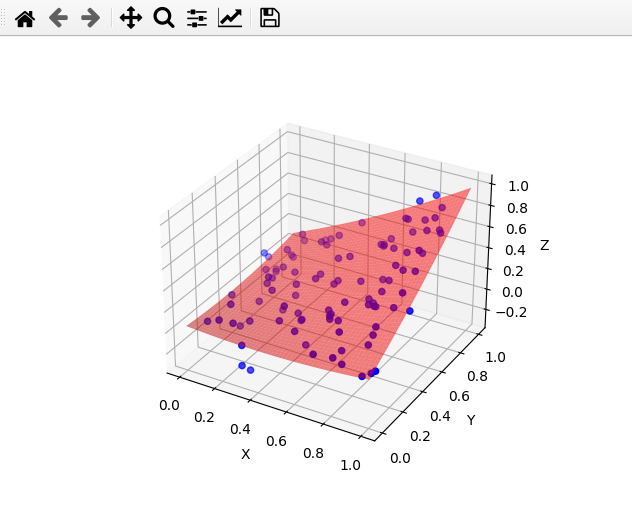
3D curve fitting

The code above creates a 3D plot of the data points and the fitted curve. The blue dots represent the original data points, and the red surface represents the fitted curve.

Full code:

so now, below is the full code which shows how we do 3D curve fitting in Python using the SciPy library.

Python3

import numpy as np
from scipy.optimize import curve_fit
import matplotlib.pyplot as plt
from mpl_toolkits.mplot3d import Axes3D

# Generate random 3D data points
x = np.random.random(100)
y = np.random.random(100)
z = np.sin(x * y) + np.random.normal(0, 0.1, size=100)
data = np.array([x, y, z]).T

# Define mathematical function for curve fitting
def func(xy, a, b, c, d, e, f):
    x, y = xy
    return a + b*x + c*y + d*x**2 + e*y**2 + f*x*y

# Perform curve fitting
popt, pcov = curve_fit(func, (x, y), z)

# Print optimized parameters
print(popt)

# Create 3D plot of the data points and the fitted curve
fig = plt.figure()
ax = fig.add_subplot(111, projection='3d')
ax.scatter(x, y, z, color='blue')
x_range = np.linspace(0, 1, 50)
y_range = np.linspace(0, 1, 50)
X, Y = np.meshgrid(x_range, y_range)
Z = func((X, Y), *popt)
ax.plot_surface(X, Y, Z, color='red', alpha=0.5)
ax.set_xlabel('X')
ax.set_ylabel('Y')
ax.set_zlabel('Z')
plt.show()

Output:

3D curve fitting 

Spline interpolation

Spline interpolation is a method of interpolation that uses a piecewise polynomial function to fit a set of data points. The interpolant is constructed by dividing the data into smaller subsets, or “segments,” and fitting a low-degree polynomial to each segment. These polynomial segments are then joined together at points called knots, forming a continuous and smooth interpolant.

The scipy library provides several functions for spline interpolation, such as interp2d and Rbf.

Python3

import numpy as np
from scipy.interpolate import Rbf
import matplotlib.pyplot as plt

# Generate random 3D data points
x = np.linspace(-5, 5, 100)
y = np.linspace(-5, 5, 100)
X, Y = np.meshgrid(x, y)
Z = np.cos(np.sqrt(X**2 + Y**2))
# Fit a radial basis function model
rbf = Rbf(X, Y, Z, function="quintic")
Z_pred = rbf(X, Y)

# Plot the original data and the fitted function
fig = plt.figure()
ax = fig.add_subplot(projection="3d")
ax.plot_surface(X, Y, Z)
ax.plot_surface(X, Y, Z_pred)
plt.show()

Output:

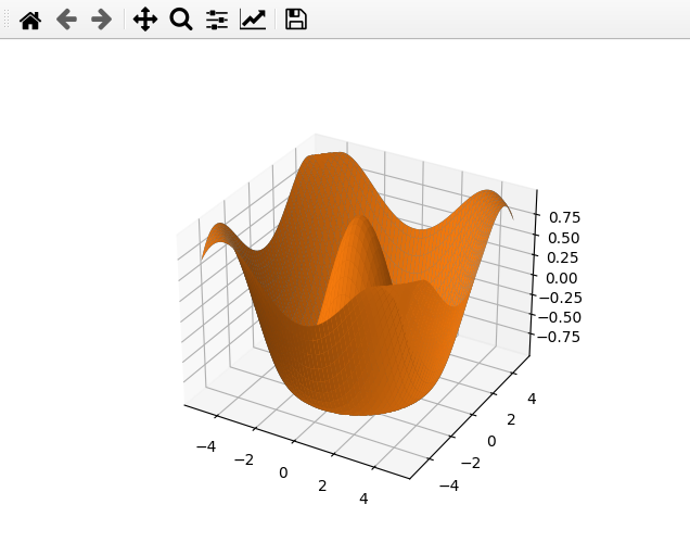
Spline interpolation

In this article, we have discussed how to perform 3D curve fitting in Python using the SciPy library. We have generated some random 3D data points, defined a polynomial function to be used for curve fitting, and used the curve_fit function to find the optimized parameters of the function. We then used these parameters to plot the fitted curve in 3D space.

Curve fitting is a powerful technique for data analysis and mathematical modeling, and Python provides several libraries that make it easy to perform curve fitting. The SciPy library is a popular choice for curve fitting in Python, and it provides several functions that can be used for curve fitting in 1D, 2D, and 3D space.