SciPy | Curve Fitting

Given a Dataset comprising of a group of points, find the best fit representing the Data.
We often have a dataset comprising of data following a general path, but each data has a standard deviation which makes them scattered across the line of best fit. We can get a single line using curve-fit() function. 
Using SciPy : 
Scipy is the scientific computing module of Python providing in-built functions on a lot of well-known Mathematical functions. The scipy.optimize package equips us with multiple optimization procedures. A detailed list of all functionalities of Optimize can be found on typing the following in the iPython console: 

help(scipy.optimize)

Among the most used are Least-Square minimization, curve-fitting, minimization of multivariate scalar functions etc.
Curve Fitting Examples – 
Input : 

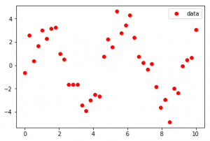
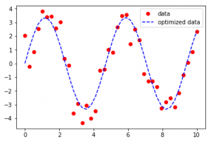
Output : 

Input : 

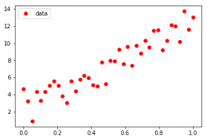
Output : 

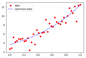
As seen in the input, the Dataset seems to be scattered across a sine function in the first case and an exponential function in the second case, Curve-Fit gives legitimacy to the functions and determines the coefficients to provide the line of best fit.

Code showing the generation of the first example – 

Python3

import numpy as np

# curve-fit() function imported from scipy
from scipy.optimize import curve_fit

from matplotlib import pyplot as plt

# numpy.linspace with the given arguments
# produce an array of 40 numbers between 0
# and 10, both inclusive
x = np.linspace(0, 10, num = 40)


# y is another array which stores 3.45 times
# the sine of (values in x) * 1.334.
# The random.normal() draws random sample
# from normal (Gaussian) distribution to make
# them scatter across the base line
y = 3.45 * np.sin(1.334 * x) + np.random.normal(size = 40)

# Test function with coefficients as parameters
def test(x, a, b):
    return a * np.sin(b * x)

# curve_fit() function takes the test-function
# x-data and y-data as argument and returns
# the coefficients a and b in param and
# the estimated covariance of param in param_cov
param, param_cov = curve_fit(test, x, y)


print("Sine function coefficients:")
print(param)
print("Covariance of coefficients:")
print(param_cov)

# ans stores the new y-data according to
# the coefficients given by curve-fit() function
ans = (param[0]*(np.sin(param[1]*x)))

'''Below 4 lines can be un-commented for plotting results
using matplotlib as shown in the first example. '''

# plt.plot(x, y, 'o', color ='red', label ="data")
# plt.plot(x, ans, '--', color ='blue', label ="optimized data")
# plt.legend()
# plt.show()

Output:

Sine function coefficients:
[ 3.66474998  1.32876756]
Covariance of coefficients:
[[  5.43766857e-02  -3.69114170e-05]
 [ -3.69114170e-05   1.02824503e-04]]

Second example can be achieved by using the numpy exponential function shown as follows: 

Python3

x = np.linspace(0, 1, num = 40)

y = 3.45 * np.exp(1.334 * x) + np.random.normal(size = 40)

def test(x, a, b):
    return a*np.exp(b*x)

param, param_cov = curve_fit(test, x, y)

However, if the coefficients are too large, the curve flattens and fails to provide the best fit. The following code explains this fact:

Python3

import numpy as np
from scipy.optimize import curve_fit

from matplotlib import pyplot as plt

x = np.linspace(0, 10, num = 40)

# The coefficients are much bigger.
y = 10.45 * np.sin(5.334 * x) + np.random.normal(size = 40)

def test(x, a, b):
    return a * np.sin(b * x)

param, param_cov = curve_fit(test, x, y)

print("Sine function coefficients:")
print(param)
print("Covariance of coefficients:")
print(param_cov)

ans = (param[0]*(np.sin(param[1]*x)))

plt.plot(x, y, 'o', color ='red', label ="data")
plt.plot(x, ans, '--', color ='blue', label ="optimized data")
plt.legend()
plt.show()

Output:

Sine function coefficients:
[ 0.70867169  0.7346216 ]
Covariance of coefficients:
[[ 2.87320136 -0.05245869]
 [-0.05245869  0.14094361]]

The blue dotted line is undoubtedly the line with best-optimized distances from all points of the dataset, but it fails to provide a sine function with the best fit.
Curve Fitting should not be confused with Regression. They both involve approximating data with functions. But the goal of Curve-fitting is to get the values for a Dataset through which a given set of explanatory variables can actually depict another variable. Regression is a special case of curve fitting but here you just don’t need a curve that fits the training data in the best possible way(which may lead to overfitting) but a model which is able to generalize the learning and thus predict new points efficiently.