How to do exponential and logarithmic curve fitting in Python?

In this article, we will learn how to do exponential and logarithmic curve fitting in Python. Firstly the question comes to our mind What is curve fitting?

Curve fitting is the process of constructing a curve or mathematical function, that has the best fit to a series of data points, possibly subject to constraints.

• Logarithmic curve fitting: The logarithmic curve is the plot of the logarithmic function.
• Exponential curve fitting: The exponential curve is the plot of the exponential function.

Let us consider two equations 

y = alog(x) + b where a ,b  are coefficients of that logarithmic equation.

y = e^(ax)*e(b)  where a ,b  are coefficients of that exponential  equation.

We will be fitting both curves on the above equation and find the best fit curve for it. For curve fitting in Python, we will be using some library functions

• numpy
• matplotlib.pyplot

We would also use numpy.polyfit() method for fitting the curve. This function takes on three parameters x, y and the polynomial degree(n) returns coefficients of nth degree polynomial.

Syntax: numpy.polyfit(x, y, deg)

Parameters:

• x->x-coordinates
• y->y-coordinates
• deg -> Degree of the fitting polynomial. So, if deg is given one we get coefficients of linear polynomial or if it is 2 we get coefficients of a quadratic polynomial.

Logarithmic curve fitting

To do Logarithmic curve fitting, we have to follow some steps which are explained below with the implementation.

Importing Libraries

Python

import numpy as np

# It is for plotting the curve
import matplotlib.pyplot as plt

Creating/Loading Data

As we have imported the required libraries we have to create two arrays named x and y. And after creating those two arrays we have to take the log of the values in x and y with the help of numpy.log() method.

Python3

# Points on X-axis
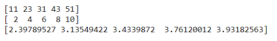
x_data = np.array([11, 23, 31, 43, 51])

# Points on Y-axis
y_data = np.array([2, 4, 6, 8, 10])

print(x_data)
print(y_data)

# Taking log of x values
xlog_data = np.log(x_data)

print(xlog_data)

Output:

Fitting of Data

After, getting the log values of x and y arrays, With the help of numpy.polyfit() we find the coefficient for our equation. As we took a linear equation hence in polyfit method we will pass 1 in degree parameter.

Python3

# Given log values of x , y as input
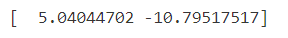
curve = np.polyfit(log_x_data, y_data, 1)

print(curve)

Output:

Getting Output

So we get the coefficients as [5.04, -10.79] with that we can get the equation of the curve which would be (y= a*log(x)+y, where a,b are  coefficient)

y = 5.04*log(x) - 10.79

Python3

y = 5.04 * log_x_data - 10.79

print(y)

Output:

Plotting Results

Now, let’s plot the graphs one with xlog_data, ylog_data, and another with xlog_data and y equation which we have obtained. For plotting graphs in python, we will take the help of Matplotlib.pyplot.plot() function.

Syntax: matplotlib.pyplot.plot(x-coordinates, y-coordinates)

Parameters:

• x: horizontal coordinates of the data points
• y: vertical coordinates of the data points

Python3

# Blue color
plt.plot(log_x_data, y_data)

# Best fit in orange
plt.plot(log_x_data, y)

Output:

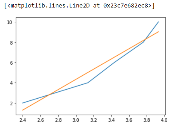
In the above graph yellow line represents the graph of original x and y coordinates and the blue line is the graph of coordinates that we have obtained through our calculations, and it is the best fit.

Exponential curve fitting

We will be repeating the same process as above, but the only difference is the logarithmic function is replaced by the exponential function.

First, let us create the data points

Python3

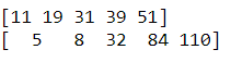
x_data = np.array([11, 19, 31, 39, 51])
print(x_data)

y_data = np.array([5, 8, 32, 84, 110])
print(y_data)

Output:

Equation: y = e(ax)*e(b)

In this equation we will plot the graph and the a, b are coefficients which we can be obtained with numpy.polyfit() method. Now lets us find the coefficients of exponential function with degree .

Python3

ylog_data = np.log(y_data)
print(ylog_data)

curve_fit = np.polyfit(x_data, log_y_data, 1)
print(curve_fit)

Output:

So, a = 0.69 and b = 0.085 these are the coefficients we can get the equation of the curve which would be (y = e^(ax)*e^(b), where a, b are coefficient)

y = e(0.69x)*e(0.085)  final equation. 

Python3

y = np.exp(0.69) * np.exp(0.085*x_data)

print(y)

Output:

Now, let us plot the graphs with the help of Matplotlib.pyplot.plot() function.

Python3

# Blue
plt.plot(x_data, y_data)

# best fit in orange
plt.plot(x_data, y)

Output:

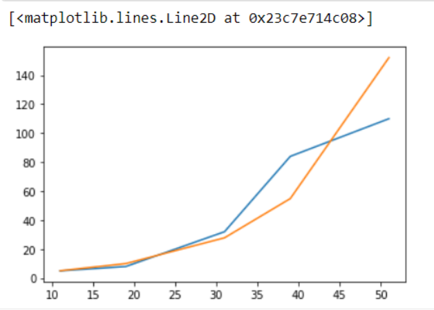
In the above graph blue line represents the graph of original x and y coordinates and the orange line is the graph of coordinates that we have obtained through our calculations, and it is the best fit.

Hence, this is the process of fitting exponential and logarithmic curves in Python with the help of NumPy and matplotlib.